Machine learning potentials for complex aqueous systems made simple
Machine-learned potentials are usually built to be general, and generality is what makes them expensive to produce. GAP-20 is cited in this paper as an example of that approach: a training database assembled over years, covering a whole element’s chemical space, with the hyperparameter scans and the sampling strategy to match.
The argument here is that most scientific questions do not need a model like that. They need one that is correct at a single thermodynamic state point, for a single system, and such a model can be built in a few days with almost no human input. The interesting part is not that this is possible in principle but that it can be made routine: the same protocol, unchanged, applied to six chemically dissimilar systems.
What we built
A committee neural network potential: several Behler–Parrinello networks trained from independent random initialisations on overlapping subsets of the same data. The committee mean is the prediction. The spread between members is a calibrated estimate of the model’s own error, and that error estimate is what drives everything downstream.
The active learning loop starts from twenty randomly chosen frames of one short ab initio trajectory. Train the committee, then repeatedly add the twenty frames on which the members disagree most about the atomic forces. The loop needs no new electronic structure calculations at any point, because the reference trajectory already carries energies and forces for every frame, so the expensive step happened once, before the loop began. Convergence arrives at roughly 300 training structures.
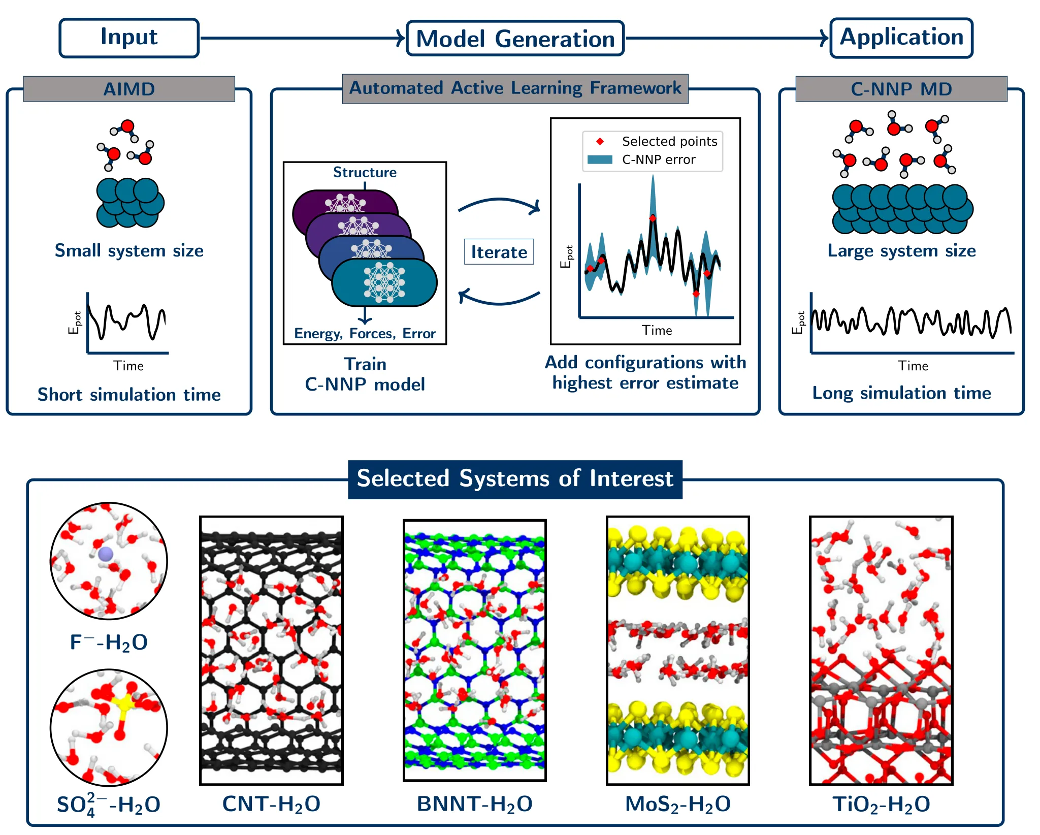
The protocol, and the six systems it was applied to unchanged. A short ab initio trajectory goes in at the top; the committee is grown by query-by-committee selection in the middle; long simulation comes out at the bottom. The systems below span solvated ions, two flavours of nanoconfinement and an oxide interface, chosen to have as little in common as possible.
Fig. 1 from Schran, Thiemann, Rowe, Müller, Marsalek and Michaelides, Proc. Natl. Acad. Sci. U.S.A. 118, e2110077118 (2021). CC BY-NC-ND 4.0.
The six systems are fluoride and sulfate ions in solution, water inside carbon and boron nitride nanotubes, water confined between MoS₂ sheets, and water on rutile TiO₂(110). No per-system hyperparameter tuning was performed. An automated protocol scores each model against its own reference trajectory on radial distribution functions, vibrational density of states and force RMSE, so the assessment is as uniform as the training.
What it showed
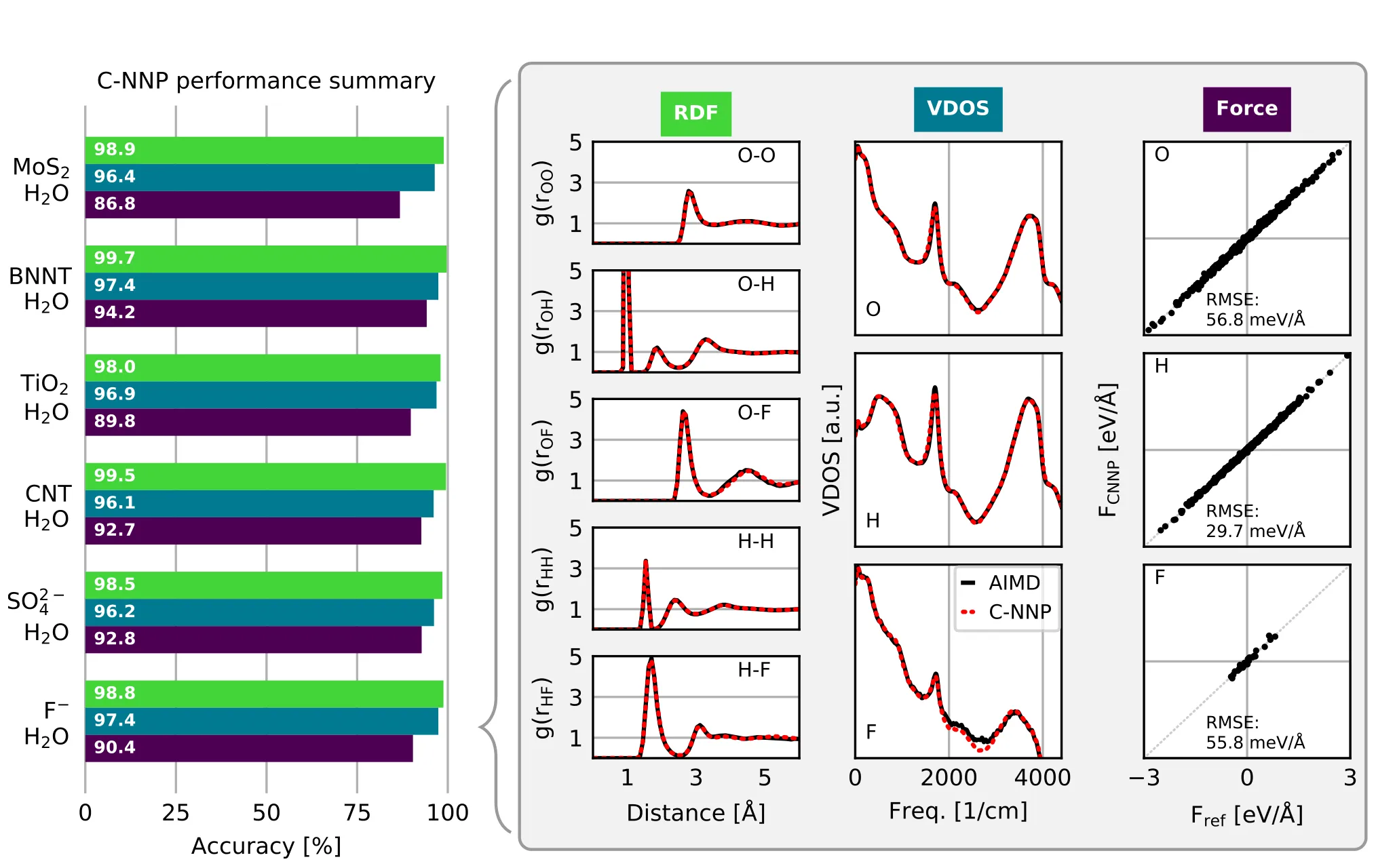
Across all six systems, RDF scores of 98–100%, VDOS 96–98%, and force agreement of 86–95%. For the fluoride–water model the force RMSE is 56.8 meV Å⁻¹ on oxygen, 29.7 on hydrogen and 55.8 on fluorine. The resulting potentials are four to five orders of magnitude cheaper than the DFT they replace, and it is that margin, not the accuracy on its own, that buys the applications.
Water on rutile TiO₂(110) is where the paper spends it: 5 ns of dynamics on 1728 atoms, which is roughly three orders of magnitude more sampling than the equivalent ab initio calculation could deliver. The density profile resolves two sharp contact layers, diffusion in the strongly adsorbed first layer is essentially zero, and the interface perturbs water diffusion more than a nanometre into the liquid.
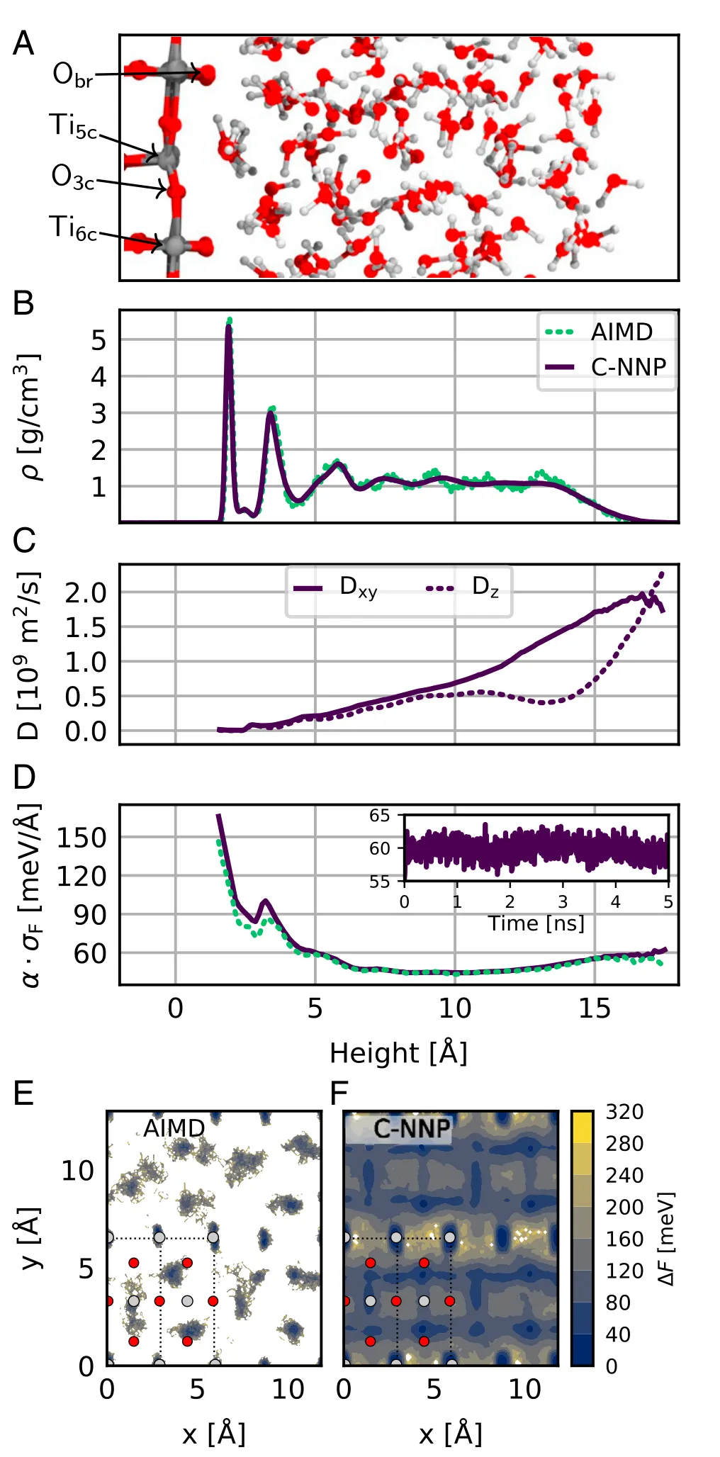
Water on rutile TiO₂(110). Panels E and F are the same adsorption free energy map computed from ab initio dynamics and from the committee potential: the first has too little statistics to resolve the minima, the second is converged. Panel D is the argument for carrying a committee at all. The model’s own error estimate, resolved against distance from the surface, stays between 40 and 80 meV Å⁻¹ across the whole water region and does not drift over the trajectory.
Fig. 3 from Schran, Thiemann, Rowe, Müller, Marsalek and Michaelides, Proc. Natl. Acad. Sci. U.S.A. 118, e2110077118 (2021). CC BY-NC-ND 4.0.
That last point deserves emphasis, because it is the difference between a fast model and a usable one. A single neural network potential run for 5 ns gives no indication of whether it has wandered somewhere its training set does not cover; the trajectory looks the same either way. A committee reports its own uncertainty continuously and at no meaningful extra cost, which turns “the simulation ran” into “the simulation stayed inside the model’s domain of validity for its whole length”.
Contribution
Third author, sharing equal-contribution credit with Fabian Thiemann. My part was the model generation and its application across the six systems; the AML active-learning package it runs on is Schran and Marsalek’s.
What the models were spent on
This is the methodological half of a longer run of work on solid–liquid interfaces, and the protocol only earns its keep in what came after it.
The nanotube systems here were demonstrations. A year later they became the object of study in their own right, scaled from a single (12,12) tube to sixteen tubes up to 5.5 nm across and over forty nanoseconds of dynamics, which is what it took to separate the geometric part of nanotube friction from the chemical part.
Alongside that ran the collaborations with Rahul Nair’s experimental group at the National Graphene Institute in Manchester, on vermiculite membranes and later MoS₂ membranes. Those ran at direct ab initio cost rather than through a learned potential, but they belong to the same thread and they followed a consistent pattern: the experimentalists had a clean anomaly they could measure and could not explain, and wanted a mechanism rather than a curve fit. Both ended up hinging on the structure of a nanometre or two of confined water.
Two things came out of that stretch of work, and neither is about water.
The first is that the useful unit here was a protocol rather than a model. A model someone else has to refit before they can use it does not travel; a procedure that reliably produces a working model in a few days does. Which is the same argument GAP-20 makes about publishing the artefact, arrived at from the opposite end.
The second is that the hardest part of an interdisciplinary collaboration is agreeing what question the simulation is answering. The MoS₂ work is the good example: the informative result was a negative one, that lithium loading does not change how fast water diffuses in an open channel, and a negative only counts as an answer if the question was sharpened enough beforehand for it to eliminate something.
Where this sits
It builds directly on Schran, Brezina and Marsalek’s committee neural network potentials from the previous year, which established that committee disagreement tracks generalisation error closely enough to drive active learning. This paper is the application layer on top of that result.
Read alongside GAP-20, the two form a coherent sequence rather than a contradiction: build the general-purpose potential, establish what it costs in effort and in accuracy, then make the case for a cheap state-point-specific alternative where generality is not what the question requires.