2025

Atomic orbitals, computed and drawn properly

Method Vectorised evaluation of hydrogenic wavefunctions on an xarray grid, marching cubes for isosurfaces System One-electron atomic orbitals at arbitrary n, l and m Result Coarse evaluation, interpolation, then a smooth isosurface. Pure Python, no viewer

Almost every orbital picture you have seen is a drawing. Someone looked at the analytic form, decided roughly what shape it implied, and drew that. Which is why the four lobes of a d orbital are so often identical, so often symmetric, and so often subtly wrong about where the density actually goes.

The wavefunctions are known in closed form. There is no reason to draw them by hand.

What it does

Give it three quantum numbers and it evaluates the one-electron wavefunction on a three-dimensional grid, then renders the probability density either as a point cloud or as a marching-cubes isosurface. Cartesian and spherical implementations sit behind the same interface, so you can pick whichever is natural for what comes next: Cartesian for plotting, spherical if the result is feeding a calculation with physical meaning.

The grid is an xarray object and every evaluation is vectorised, which matters more than it sounds like: a naive triple loop over a 100³ grid is unusably slow in Python, and the whole point of the exercise was that generating a new orbital should take seconds, not minutes.

The one deliberate trick is decoupling accuracy from appearance. Isosurfaces need a fine grid to look smooth, but a fine grid is expensive and the extra points buy nothing physically. So the wavefunction is evaluated on a coarse grid and interpolated up before rendering. Anything quantitative uses the coarse values; only the picture uses the interpolated ones. Mixing those up would be an easy way to publish a very smooth lie, so the two paths stay separate and the docs say which is which.

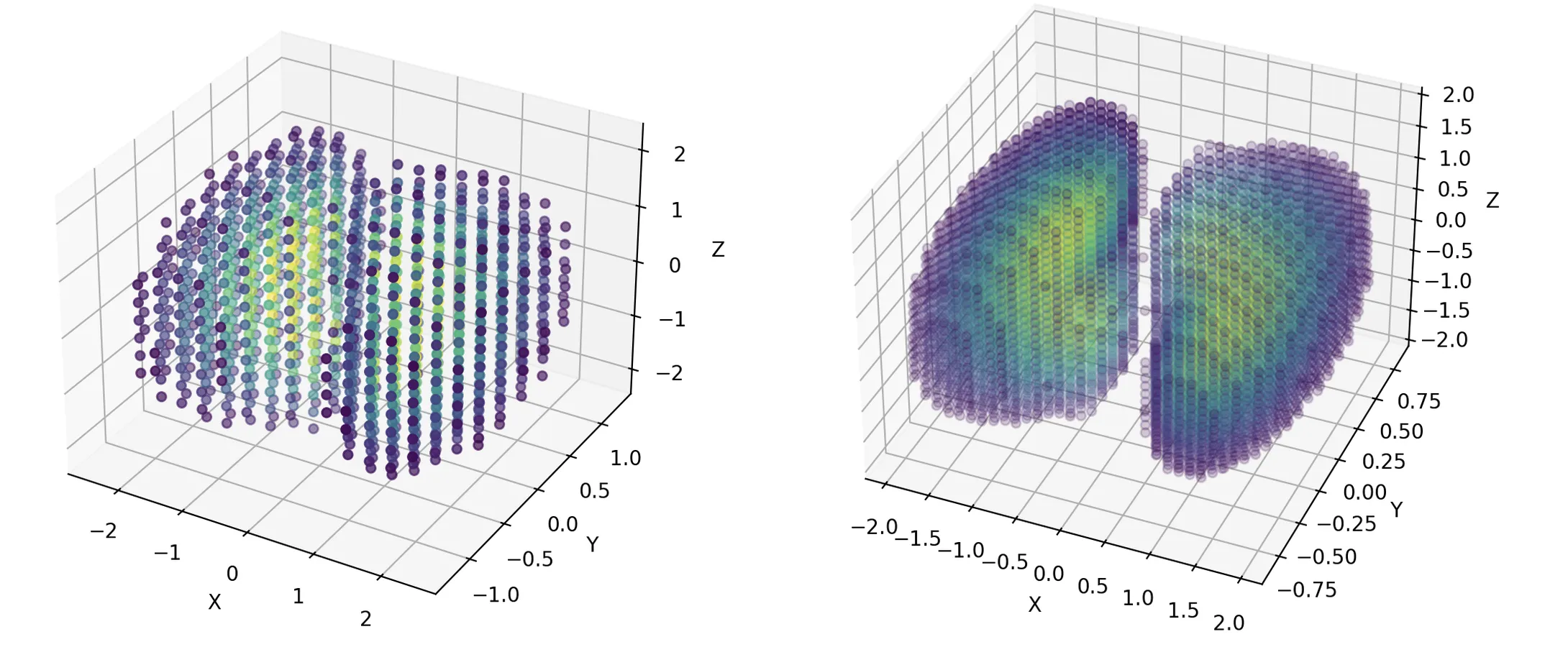
Two three-dimensional scatter plots of the 2p orbital probability density. On the left a sparse 20-cubed grid of coloured points; on the right the same wavefunction interpolated to a 50-cubed grid, where the two lobes are dense and continuous. — Fig. 1
The 2p orbital evaluated on a 20³ grid (left) and the same values interpolated up to 50³ (right), both drawn as point clouds coloured by probability density. The left panel is what was actually computed and the only one anything quantitative should use. The right panel is the picture. Nothing was added between them except interpolation, which is exactly why the two have to stay labelled. Own work, from the project’s own examples.

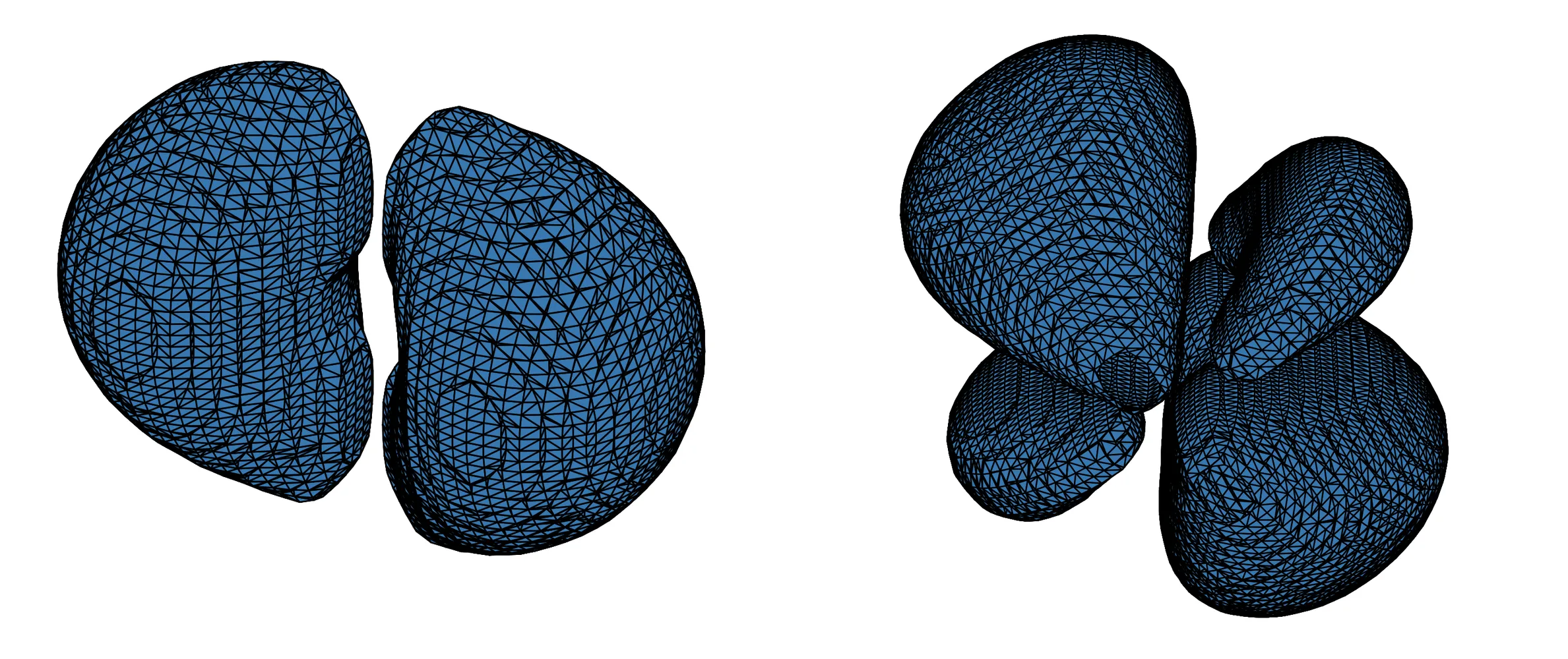
Two marching-cubes isosurfaces rendered as triangulated meshes: the two-lobed 2p orbital on the left, and the 4d-z-squared orbital on the right with two large axial lobes and a torus around the middle. — Fig. 2
Isosurfaces of the 2p orbital (left) and the 4d_z² orbital (right), both drawn by marching cubes at a fixed fraction of the maximum density. The triangulation is left visible rather than smooth-shaded, so the resolution of the underlying grid is legible in the picture instead of being hidden by it. The 4d_z² lobes are not the identical footballs of the textbook diagram. Own work, from the project’s own examples.

Why bother

Partly because it is a satisfying afternoon’s work, and partly for a reason that generalises: this is the smallest possible version of a problem that shows up constantly in computational chemistry. You have an expensive function on a grid, you need it accurate somewhere and merely pretty somewhere else, and confusing the two is how wrong pictures end up in papers.

It also has tests, which is unusual for a plotting side project and was the point.

Code ↗