Machine learning potentials for carbon
Carbon is several materials wearing one element. Diamond, graphite, graphene, nanotubes, fullerenes, amorphous films and the hot liquid differ enough in their bonding that a model fitted to any one of them is usually wrong about the rest, and the standard models were fitted to a few of them by hand. Anyone who has simulated a carbon material with more than a few hundred atoms for longer than a few picoseconds has used one of those models, and has inherited its opinions. Some of the opinions are odd. Ask the classical carbon potentials of 2017 (fitted formulas that give the energy of a set of atoms, and the forces on them, from their positions) whether a free graphene sheet expands or contracts when you warm it, and they disagree on the sign: three of them switch sign somewhere between 500 and 1000 K, one tears the sheet apart above 1500 K, and none of them agrees with the quantum-mechanical answer across the whole range. Thermal expansion is about as basic as a property gets.
This article is about the years from 2016 to 2022 that I spent replacing those opinions with a fitted one, first for graphene alone and then for every form of carbon at once, and about what happened when these potentials were run at scale, by other people and by me. The short version: one machine-learned model can cover the whole element while keeping graphene’s vibrations within 4 meV of density functional theory (DFT, the quantum-mechanical method the machine-learned models are fitted to); a benchmark led by others later ranked it first of seven potentials on clusters it had not been trained for; and 5,832 atoms of hot carbon told me that whether a network graphitises (turns into sheets of hexagons, as in graphite) is decided by its density and hardly at all by its temperature. The long version follows in two halves: build the potentials, then use them.
Graphene potential
Graphene is the form of carbon everyone has heard of, and on paper the simplest one to start with: a single sheet of hexagons with one bond length and one angle. Reproducing the structure at 0 K is the easy part, though. The properties people measure, the thermal expansion, the phonon spectrum (the sheet’s vibrational frequencies), the Raman shift (a vibrational frequency read from scattered light) with temperature, come from how the energy changes as the sheet bends and stretches, and that is where a model fitted by hand to a handful of numbers has nothing to say. So the question I set out to answer in 2017, with Gábor Csányi at the University of Cambridge’s Engineering Laboratory, and Dario Alfè and Angelos Michaelides at University College London (UCL), who supervised the PhD, was narrower than it sounds. It was whether a potential fitted to DFT forces, with no physics put in by hand beyond the choice of descriptors (the numbers that encode an atom’s surroundings), could stand in for ab initio molecular dynamics (AIMD, in which atoms move step by step under forces computed with DFT) on graphene, and how far behind it the potentials people use every day would fall.
The method was the Gaussian approximation potential (GAP): the energy of an atom is written as a sum of a two-body term, a three-body term and a many-body term built on the smooth overlap of atomic positions (SOAP) descriptor, each term a Gaussian-process fit to a set of reference environments (a regression that predicts a new environment from its similarity to the reference ones), all with a 4.0 Å cutoff. The reference data came from VASP (a plane-wave DFT code) with the optB88-vdW functional (a form of DFT that includes van der Waals attraction), converged tightly to keep the noise in the forces low. As important as any hyperparameter (a setting chosen before the fit) was where the training configurations came from. Three molecular dynamics (MD) runs at 1000, 2000 and 3000 K under an existing empirical potential, LCBOP, seeded the first 300. From there the model bootstrapped itself: each new GAP drove its own dynamics, the configurations it visited were computed with DFT and added, and the fit was repeated, until the final training set held 1,083 sheets of 200 atoms spanning 300–4000 K and a small range of lattice parameters (the repeat distance of the hexagonal lattice). A potential trained this way has seen the places it will go. That is the whole trick.
The benchmark was the crowded field: density functional tight binding (DFTB, an approximate quantum method), ReaxFF, Tersoff, REBO, AIREBO, AIREBO-Morse, LCBOP and the amorphous-carbon GAP of Volker L. Deringer and Csányi, all run on the same tests. On forces the contest was not close. Against a sample of 15,000 DFT reference forces the graphene GAP made a root-mean-square error (RMSE) of 0.028 eV Å⁻¹ in the plane of the sheet and 0.019 eV Å⁻¹ out of it; the best empirical potential in the plane, AIREBO, sat at 0.548 eV Å⁻¹, twenty times higher, and Tersoff at 3.122 eV Å⁻¹, with individual errors above 11 eV Å⁻¹. Out of the plane the best of the rest, DFTB at 0.162 eV Å⁻¹, had eight to ten times the GAP’s error. For scale, the difference between two reasonable exchange–correlation functionals on the same forces is 0.026 eV Å⁻¹ in the plane, so the GAP was as close to its own reference as one flavour of DFT is to another. The 0 K lattice parameter came out at 2.467 Å against 2.464 Å from DFT and 2.462 Å for graphite at room temperature, a 0.1% miss shared only by ReaxFF.
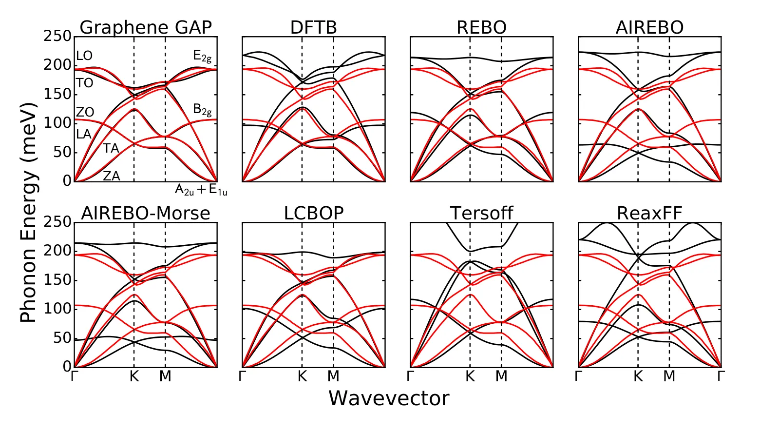
Phonon dispersion of graphene (vibrational frequency along a path through wavevector space) from each potential (lines) against the dispersion derived from X-ray diffraction on graphite (points). The machine-learned potential sits within a millielectronvolt of the reference at almost every high-symmetry point (the labelled points on the horizontal axis); every empirical potential misses the longitudinal optical branch (the highest-frequency branch), Tersoff by 110 meV at the Γ point (the long-wavelength limit). Reproduced from Rowe et al., Phys. Rev. B 97, 054303 (2018), figure 3. Copyright 2018 American Physical Society; used under the authors’ right to reuse on their own website.
Forces are the currency a potential is fitted in, so a good force error is the least you should expect. The properties are the test. The phonon dispersion is the one I would show anyone who doubts that a fitted model can carry real physics: against the dispersion derived from X-ray diffraction on graphite, the GAP is within a millielectronvolt at almost all of the high-symmetry points, where REBO, AIREBO, AIREBO-Morse and Tersoff make mean absolute errors of 10, 20, 20 and 40 meV, and every empirical model gets the highest branch wrong. That branch is the longitudinal optical one, the stiffest vibration in the sheet, and the classical models either soften it or stiffen it by 20 to 110 meV. The Raman G band, which is that vibration seen at the zone centre (the Γ point), softens with temperature in the experiments once the strain from the substrate is corrected out, and the GAP follows the measurements across the 150–900 K they cover.
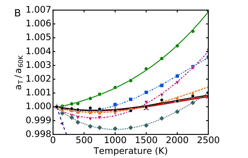
In-plane thermal expansion of a free graphene sheet from 60 to 2500 K: the lattice parameter relative to each model’s own 60 K value, from constant-pressure ab initio molecular dynamics and from each potential (panel B of the paper’s figure 2). The ab initio lattice parameter changes by 0.1% across the whole range; only the machine-learned potential tracks it. Reproduced from Rowe et al., Phys. Rev. B 97, 054303 (2018), figure 2, panel B. Copyright 2018 American Physical Society; used under the authors’ right to reuse on their own website.
Thermal expansion is where the empirical potentials fall over in public. Constant-pressure AIMD on the free sheet, three runs per temperature from 60 to 2500 K, changes the in-plane lattice parameter by 0.1% over the whole range, which is to say it barely moves, and the GAP follows it in absolute and in relative terms. LCBOP, AIREBO and AIREBO-Morse have the coefficient of thermal expansion change sign between 500 and 1000 K; ReaxFF fragments the sheet above 1500 K. No empirical potential in the set predicts both the 0 K lattice parameter and the finite-temperature expansion, and the paper says so. REBO is the best of them overall, and REBO costs 1.2 times what Tersoff does.
The price of the GAP is compute. Per MD step on 200 atoms it costs 340 times what Tersoff costs, less than DFTB at 950, and about four orders of magnitude less than AIMD for the same system. And the paper says one more thing plainly that I want to repeat, because the next section depends on it: the model is not transferable to other phases of carbon (it does not carry over beyond the kinds of structure it was trained on). Its training set held nothing but graphene, so it cannot describe diamond. That is not a bug in a specialist model. It is the reason a specialist model is not enough.
GAP-20
The GAP-20 paper frames the problem with two earlier potentials, and they were opposites. The graphene model above was accurate and narrow. GAP-17, Volker Deringer and Gábor Csányi’s model for amorphous carbon, was the flexible one, made for the disordered phase. The question for GAP-20 was whether one model could have both, the flexibility of the amorphous potential and the numerical accuracy of the graphene one, for every form of carbon at once, and what that would cost. The work was mine as first author, with Volker Deringer, then at the University of Oxford, Piero Gasparotto at UCL, Gábor Csányi in Cambridge and Angelos Michaelides at UCL, and it is the second of the two papers in my PhD thesis.
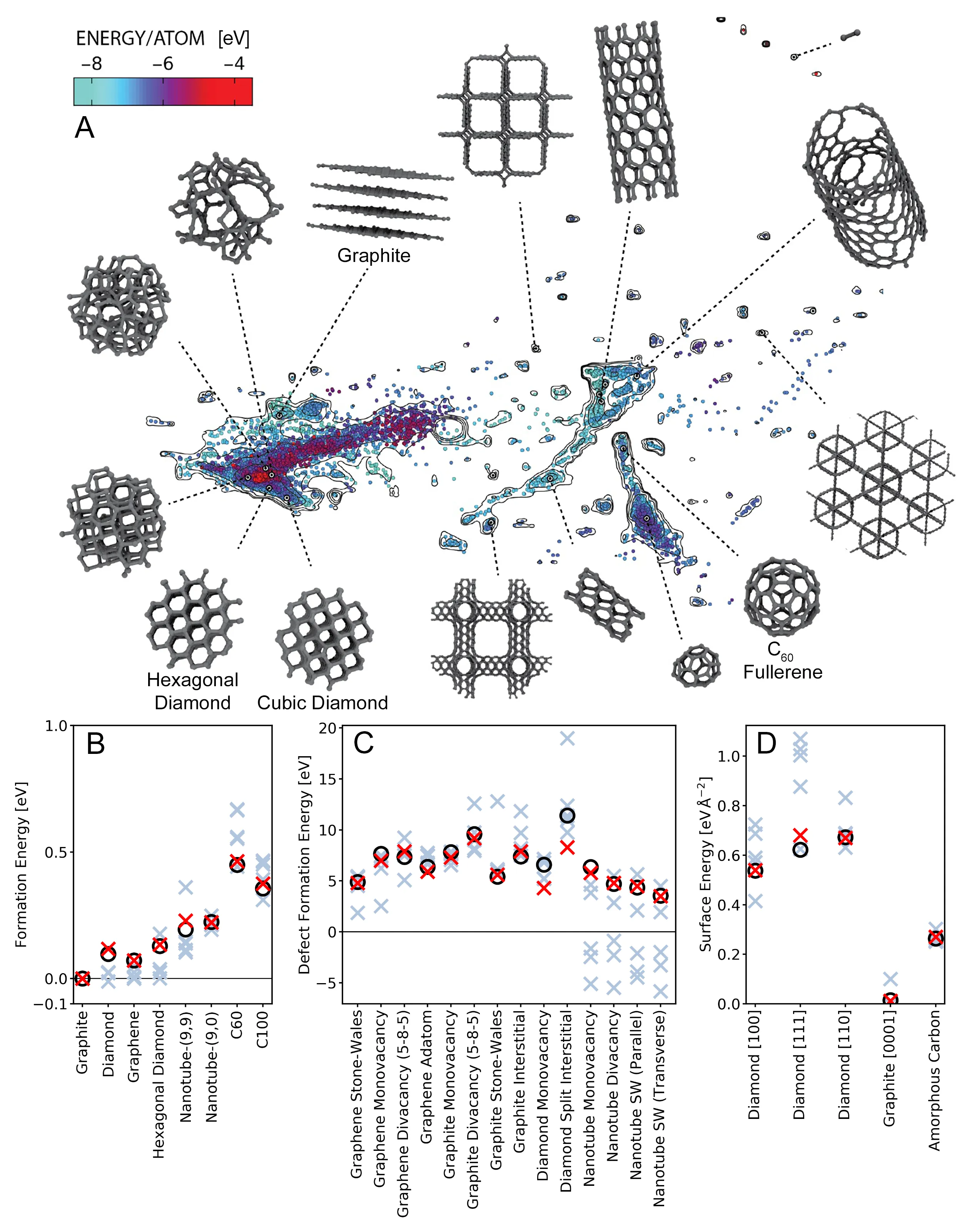
The GAP-20 database as a sketch-map: a two-dimensional projection of the SOAP similarity between atomic environments, one point per environment, with representative structures drawn around it. Crystals, surfaces, defects, fullerenes, nanotubes, the liquid and amorphous carbon occupy their own regions, and the model is fitted to all of them at one level of theory. Panels B to D put GAP-20 (red crosses) and DFT (black circles) side by side on the formation energies of the crystalline allotropes, the defect formation energies and the surface energies, with the empirical potentials (pale crosses) scattered around them. Reproduced from Rowe et al., J. Chem. Phys. 153, 034702 (2020), figure 1, with the permission of AIP Publishing.
The database is the model, so most of the paper is about the database. It started from the GAP-17 and graphene sets and added every crystalline phase, every fullerene under 240 atoms, nanotubes with chiral indices from 3 to 10 in cells under 240 atoms, the SACADA catalogue of allotropes (structural forms of the element), the structures GAP-17 had found by random structure search (relaxing random starting cells to their nearest energy minimum), low-index surfaces and a set of defects. Each was sampled with ab initio and GAP-driven MD, and everything was recomputed with one functional at one cutoff, spin-polarised optB88-vdW at 600 eV: about 17,000 configurations of 1 to 240 atoms and almost 2.5 million atomic environments. Then the fit threw most of it away. The training set is the union of three parts: 4,000 configurations chosen by farthest-point sampling (each new pick the configuration least like those already chosen), which spreads the set out instead of piling it up where the dynamics happened to linger; the whole GAP-17 set; and about 1,000 configurations added by hand to target particular properties.
A two-body GAP term below 4.0 Å hands over to a semi-analytical r⁻⁶ spline (a smooth fitted curve) from 4.0 to 10 Å, fitted to the DFT binding curve of a graphene bilayer, so the model has a long-range van der Waals tail without asking the Gaussian process to learn one. The SOAP cutoff was scanned against the force error on a held-out set (configurations kept out of the fit), and the scan is a small lesson in not trusting the minimum: the error was lowest at 2.9 Å, and the cutoff was set to 4.5 Å anyway, because graphite’s layers sit about 3.3 Å apart and a model that cannot see the next layer cannot bind it. Sparse points (the reference environments the fit is built on) were scanned the same way; the errors level off at about 1,500 and the model uses 9,000.
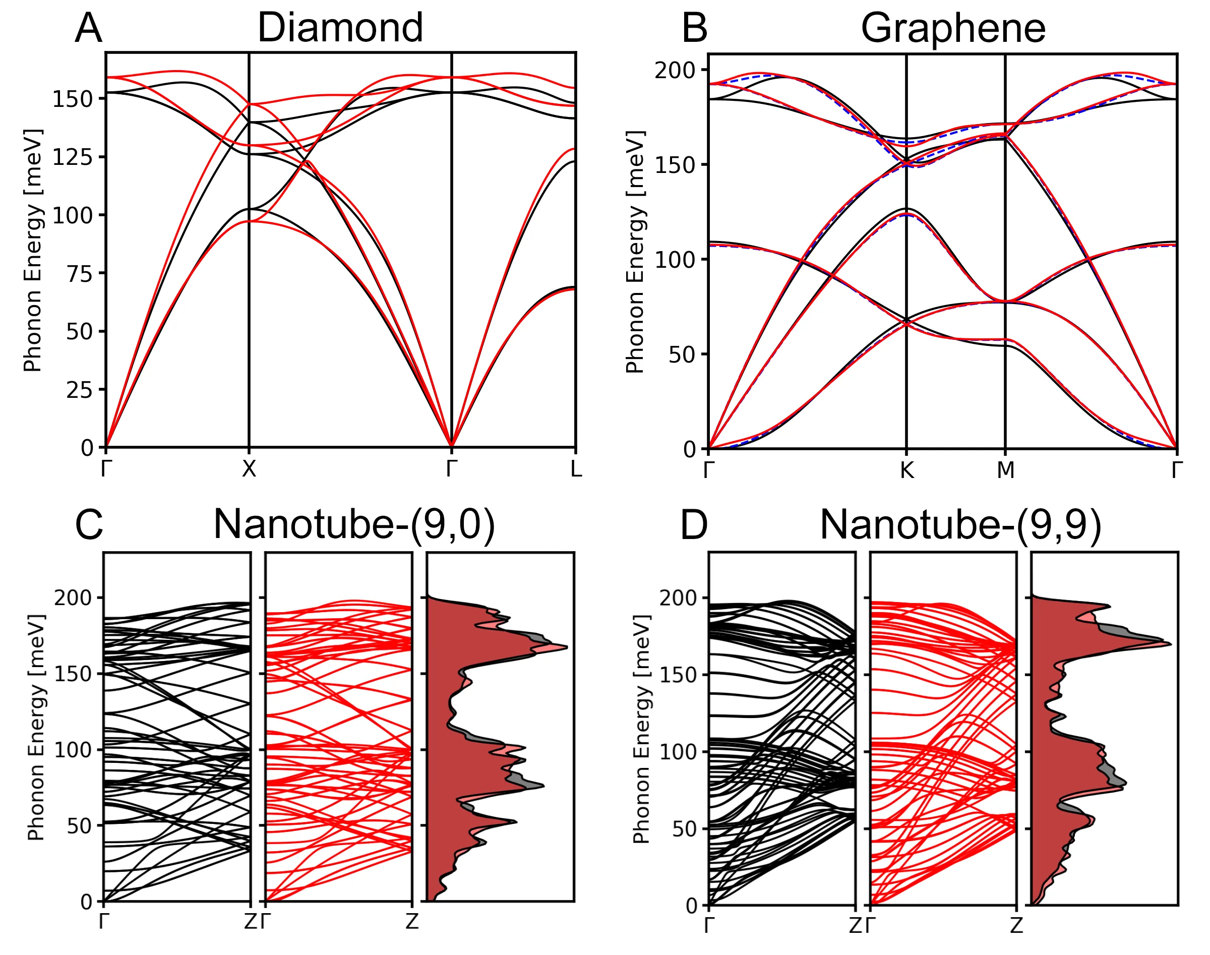
Phonon dispersions of diamond, graphene, a (9,9) armchair nanotube and a (9,0) zigzag nanotube from GAP-20 (lines) against DFT (points). The dashed line in the graphene panel is the graphene-only potential of 2018: within 1 meV of DFT at the high-symmetry points, where GAP-20 is within 4 meV, the price of covering every other form of carbon on the same footing. Reproduced from Rowe et al., J. Chem. Phys. 153, 034702 (2020), figure 5, with the permission of AIP Publishing.
So what did breadth cost? A factor of four in graphene phonon accuracy against the graphene-only model: GAP-20 keeps graphene phonons within 4 meV of DFT at the high-symmetry points, where the specialist was within 1 meV. That factor of four is the honest number for what one general model gives up against a specialist, and I would pay it every time, because on the same footing GAP-20 does diamond to within 7 meV in its stiffest modes and typical nanotube band splittings to 2–3 meV, and the graphene model was built for none of them. Across the crystalline allotropes GAP-20 gets lattice parameters and bond lengths to 0.2% on average, formation energies to 0.5% and atomisation energies (the energy to pull a structure apart into free atoms) to 1%; Tersoff, REBO-II and AIREBO make lattice errors of 5%, 4% and 1%. Tersoff and REBO-II have no interlayer binding in graphite at all, so their graphite is a stack of sheets that do not know about each other, where GAP-20 puts the c axis (the stacking repeat) at 6.71 Å against 6.65 Å from DFT.
Defects and surfaces are the harder test. Most defect formation energies land within 10% of DFT, and the relaxed geometries agree to better than 10⁻² Å in all but a handful of cases. A Stone–Wales defect in graphene, one bond rotated to make two pentagons and two heptagons, costs 4.9 eV in DFT and 4.8 eV in GAP-20; Tersoff says 1.9 eV. A monovacancy (one missing atom) in a (9,9) armchair nanotube costs 6.4 eV in DFT and 5.8 eV in GAP-20; Tersoff, REBO-II and AIREBO give −5.1, −1.6 and −2.5 eV. By their account the nanotube would rather have the hole. Diamond is the clear weak spot, with defect energies 25–35% low, and the model misses the Jahn–Teller distortion of the graphene monovacancy, a 350 meV effect that lowers the symmetry of the relaxed hole. Diamond surface energies are typically within 7%. The graphite basal surface, at 0.015 eV Å⁻² in DFT, comes out 3 meV Å⁻² off, a 20% error; LCBOP and AIREBO miss the same number by 67% and 27%.
The test I trust most is the one the model was not built for. A random structure search generated 1,000 small periodic cells, 8 atoms in a 3 Å box, relaxed every one of them with GAP-20 to a tolerance of 10⁻¹⁰ eV and then recomputed them with DFT. None of them was in the training set. All of them agreed well with DFT, and the search recovered the known structures of carbon: AB-stacked graphite lowest, then AA and ABC stacking, diamond and lonsdaleite (hexagonal diamond), the haeckelites (sheets built from five-, six- and seven-membered rings), crosslinked graphite and a structurally distinct sp¹-rich group (sp¹ carbon has two neighbours). The liquid was checked against AIMD at 5000 K across 1.5–3.5 g cm⁻³ and at 2.5 g cm⁻³ from 5000 to 9500 K; below about 3500 K the GAP-20 liquid forms a glass that slowly graphitises, a remark in the paper that turned into the graphitisation series further down this page. The model and its training data are on the Cambridge repository, the dataset under CC BY 4.0.
The thesis, and the lesson hand-picking taught
My PhD thesis, submitted to UCL and dated June 2021, holds both papers and one lesson the papers do not state as plainly. The first attempts at GAP-20 used hand-picked training data, an isolated Stone–Wales defect here, a monovacancy there, and a model trained that way performs well at exactly those state points and extremely poorly at a vacancy next to a Stone–Wales defect. Real materials are full of such combinations. The fix was to stop choosing. Many varied structures were generated stochastically instead, by GAP-driven random structure search and by MD, all of them were computed, and farthest-point sampling thinned the pile, “allowing the computer to decide” which environments were new. The thesis also claims two methodological firsts, “to the best of our knowledge” as the thesis puts it: the radially biased SOAP basis, reused since for hexagonal boron nitride and phosphorus, and the r⁻⁶ spline as a long-range term in a machine-learned potential, reused for two other layered materials. It lists the stability tests that never made a paper: liquid quenches, anneals (long holds at high temperature) of amorphous structures and surfaces, C₆₀ molecules (60-atom fullerene cages) threaded into nanotubes, nudged-elastic-band paths (lowest-energy routes between two structures) for defect formation, and cluster searches. Its cost benchmark ran diamond cells from 8 to 5,832 atoms on 72 cores; DFT gave out at 2,744 atoms, and GAP-20 will do tens of thousands of atoms for nanoseconds. Among the next steps the thesis names is carbon with hydrogen and oxygen, which is where the last section of this page picks up.
Defect corrugation
The first test of a potential is whether it agrees with the calculations it was fitted to. The second is whether someone else can find something with it. Fabian L. Thiemann, at UCL, the University of Cambridge and Imperial College London, wanted to know how much a point defect (a missing or misplaced atom or bond) changes the shape of a free graphene sheet, and whether the answer depends on which defect and how many. Free-standing graphene is never flat; it ripples. The obvious way to study defect ripples is a sheet of about 7,000 atoms at 300 K for 150 ps, which is out of reach for DFT and, as it turned out, out of reach for the classical potentials in a way worth spelling out. I was second author, with Andrea Zen at the Università di Napoli Federico II and UCL, Erich A. Müller at Imperial and Angelos Michaelides.
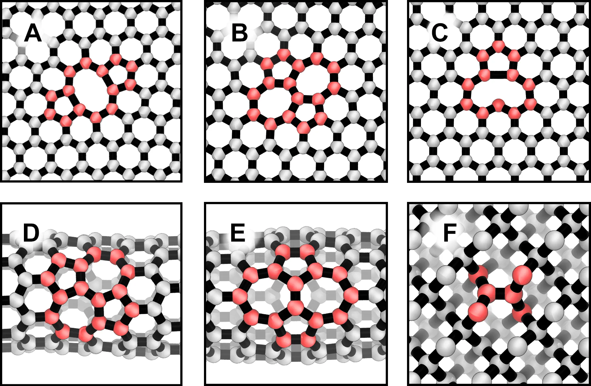
Six of the defects GAP-20 was tested on, with the atoms around each defect highlighted. The two that matter here are the graphene divacancy (panel A), two missing atoms whose neighbours reconstruct (rebond) into one eight-membered and two five-membered rings, and the Stone–Wales defect (panel B), one bond rotated by 90° into two pentagons and two heptagons. Panels C to F are the graphene monovacancy, the Stone–Wales defect in two orientations on a (9,9) nanotube, and a split interstitial in diamond. Reproduced from Rowe et al., J. Chem. Phys. 153, 034702 (2020), figure 6, with the permission of AIP Publishing.
The simulations ran in LAMMPS (an MD code) under GAP-20 at 300 K and zero stress, 20 ps of equilibration and 150 ps of statistics each, on sheets of 6,984 to 7,200 atoms with divacancies or Stone–Wales defects at concentrations from about 0.03%, an isolated defect, to 3%, where the defects sit about 1 nm apart. Defects were placed at random at least 10 Å from each other, three placements per type and concentration, and every run started from a flat sheet with unreconstructed defects, so that whatever the vacancies did to close themselves up, they did on their own. Corrugation was measured as the standard deviation of atomic heights relative to a pristine sheet under the same conditions, a ratio called the corrugation amplification factor (CAF), because absolute heights scale with the size of the sheet and the ratio does not. Around each defect a fitted height function gave its tilt and its Gaussian curvature (zero for a surface bent in one direction only, like a cylinder; negative for a saddle).
Defects roughen the sheet, and they do it early: the CAF is already well above 1 at about 0.2% and levels off above 1.5%. What decides the size of the effect is the kind of defect. At 3%, divacancies raise the CAF to almost 5 and Stone–Wales defects to almost 3, and at equal concentration a divacancy corrugates the sheet roughly twice as much as a Stone–Wales defect. The local geometry says why. A Stone–Wales defect imposes a tilt, an inclination of about 0.270 against 0.066 for three pristine hexagons, with zero Gaussian curvature, and its tilt grows by less than 20% as more defects arrive. A divacancy is a saddle, and its Gaussian curvature grows about tenfold from the isolated defect to 3%, which means the divacancies feel each other and the sheet’s shape is a collective response. For comparison, a pristine sheet squeezed by 2% corrugates about as much as a sheet with 1% defects, so the defects are doing what a modest compression would.
Now the part about potentials. LCBOP and REBO-II, run at 1% as a check, agree with GAP-20 on the trend, but only when started from divacancies that have already reconstructed. Started flat, they never get there: both overestimate the barrier to the reconstruction, and the vacancy stays an open hole. The paper’s own verdict is that “simply using these potentials without prior knowledge … is unlikely to have revealed the insights obtained here”, It found the reconstruction because the DFT it was trained on knows about the reconstruction, and nobody had to tell it.
Cluster benchmark
Benchmarks written by a model’s authors have a credibility problem, whatever the authors’ intentions, so the one I value most for GAP-20 is one designed by others. Bora Karasulu and Carla de Tomas at Happy Electron, my employer at the time, with Jean-Marc Leyssale at the University of Bordeaux and Cedric Weber at King’s College London (KCL), wanted a potential that could replace DFT in the relaxation step (moving the atoms downhill to the nearest energy minimum) of a random structure search for carbon clusters. They put seven potentials through the same search to find out which one could. I was third author.
The search was ab initio random structure searching (AIRSS), the Pickard–Needs method: random clusters of 4 to 200 atoms inside a sphere, no two atoms closer than 1.4 Å, either with no symmetry or with up to 24 symmetry operations imposed, and the same random inputs handed to each method to relax. The reference was VASP with the PBE functional (a standard form of DFT). The potentials were GAP-20 and six classical ones, all in LAMMPS: Tersoff, C-EDIP (the environment-dependent interaction potential for carbon), LCBOP-I, ReaxFF, REBO-II and AIREBO. The first finding was about the relaxation itself: the default conjugate-gradient protocol left structures with residual pressures above 100 MPa, so a FIRE stage and a truncated-Newton stage (two further minimisers) were added until the pressure was effectively zero. After duplicates, dissociated and unconverged structures were removed, DFT had 3,500 disordered and 10,500 symmetric minima to compare against, and GAP-20 had 22,200 and 20,300 of its own. The comparison was on everything a search produces: which structure is lowest at each size and what symmetry it has, the distribution of cohesive energies (energy per atom relative to free atoms), the Boltzmann-weighted coordination (number of bonded neighbours, each structure counted by its thermal population) and ring statistics at 293 K, and the radial distribution function (the spread of interatomic distances) of C₆₀.
Cohesive energy per atom of icosahedral C₆₀ from DFT and from each of the seven potentials in the benchmark, from table II of Karasulu et al. GAP-20 over-binds the molecule by 0.10 eV per atom; the six classical potentials under-bind it by between 0.30 and 0.91 eV per atom.
Own work, not published elsewhere. Made with scripts/figures/cluster_benchmark_c60.py, from table II of Karasulu et al., Carbon 191, 255–266 (2022).
GAP-20 gave the closest match to DFT on all of it: the minimum-energy structures and their point groups (their symmetries), the energy distributions, the coordination, the rings and the C₆₀ radial distribution function. The cohesive energies say it most simply. DFT and GAP-20 put the clusters between −7.5 and −6.0 eV per atom, the classical potentials between −6.5 and −4.5, and for C₆₀ itself DFT gives −7.47 eV per atom and GAP-20 −7.57, an over-binding of 0.10 eV per atom, while the classical models under-bind by 0.30 to 0.91 eV per atom. The classical potentials also failed in characteristic ways. Tersoff and LCBOP-I built surface shells of sp¹ carbon, about 35% of atoms in clusters of 30 to 200 atoms; REBO-II and AIREBO stayed trapped in the dense sp³ starting structures (sp³ carbon has four neighbours, as in diamond) they were given. GAP-20’s misses are on the record too, because that is what a benchmark is for: it puts the transition from chains to rings at C₁₀ where DFT has it at C₈, and it gets the point groups of the second- and third-lowest C₆₀ isomers wrong.
Then the authors did what the benchmark was for and searched beyond DFT’s reach, with GAP-20 alone, up to 720 atoms. The clusters stay hollow sp² cages (sp² carbon has three neighbours, as in graphite) up to about C₃₂₀, and above that the minima grow sp³ cores under faceted shells. In a low-density search of C₂₄₀ the canonical icosahedral fullerene was the minimum eight times over at −7.81 eV per atom, with octahedral pseudo-fullerenes close behind at −7.77 to −7.57, and at C₅₄₀ a fullerene-like tetrahedral cage at −7.47 eV per atom had a dense isomer within 10 meV per atom of it, a competition between the two kinds of carbon that the paper places above about C₃₂₀. The paper is candid that the fixed-radius generation makes large clusters denser than fullerenes and that these searches are not exhaustive, and it names ReaxFF as an option cheaper than GAP-20, with moderate accuracy, for anyone who cannot afford the GAP.
Graphitisation
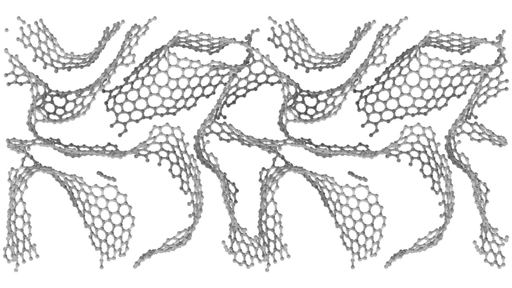
The GAP-20 paper remarks, almost in passing, that below about 3500 K its liquid carbon forms a glass that slowly graphitises. At Happy Electron in 2021 I had the compute to follow the remark up, and the question was a basic one: starting from a melt, whether the density the network is held at or the temperature it is annealed at decides if it turns graphitic. This is unpublished work of my own, presented here for the first time, and it is the source of the hero image at the top of the page.
The runs were 5,832 atoms of carbon, a 216-atom cell replicated 3 × 3 × 3, at fixed volume in LAMMPS with a 2 fs step and a Nosé–Hoover thermostat (a scheme that holds a simulation at a target temperature), driven by GAP-20, the same potential the cluster series below used.
The protocol, from the input files and logs rather than from my slides of the time, was: a short minimisation, velocities at 6000 K, a 6000 K liquid stage, a 20 ps thermostat ramp whose target starts at 300 K and rises to the anneal temperature, an anneal at the target temperature for 200 ps, and a 20 ps ramp back towards 300 K, at the end of which the frame was written with no final minimisation. In the one log I have read in full, replica one at 1.0 g cm⁻³, the system cools from 6000 K to near 1100 K on the first ramp before heating again, and ends the last ramp near 710 K. So the structures below are hot snapshots, not minima. The density set held the anneal at 3500 K and varied the density from 0.5 to 3.5 g cm⁻³ in steps of 0.5; two temperature sets held the density at 1.5 and at 3.0 g cm⁻³ and varied the anneal from 2000 to 4500 K in steps of 500 K, sharing their 3500 K member with the density set, which makes 17 conditions. Each condition was run three times, and the three replicas share a velocity seed (the random number that sets the starting velocities) and differ only in the length of the liquid stage, 20, 40 and 30 ps, so they are three cuts through one melt rather than three independent draws. That log also records 1,000 dangerous neighbour-list rebuilds (LAMMPS’s warning that atoms moved far enough between list updates for some interactions to be missed) in the liquid stage and 9,847 in the anneal, which as of September 2026 I have not chased.
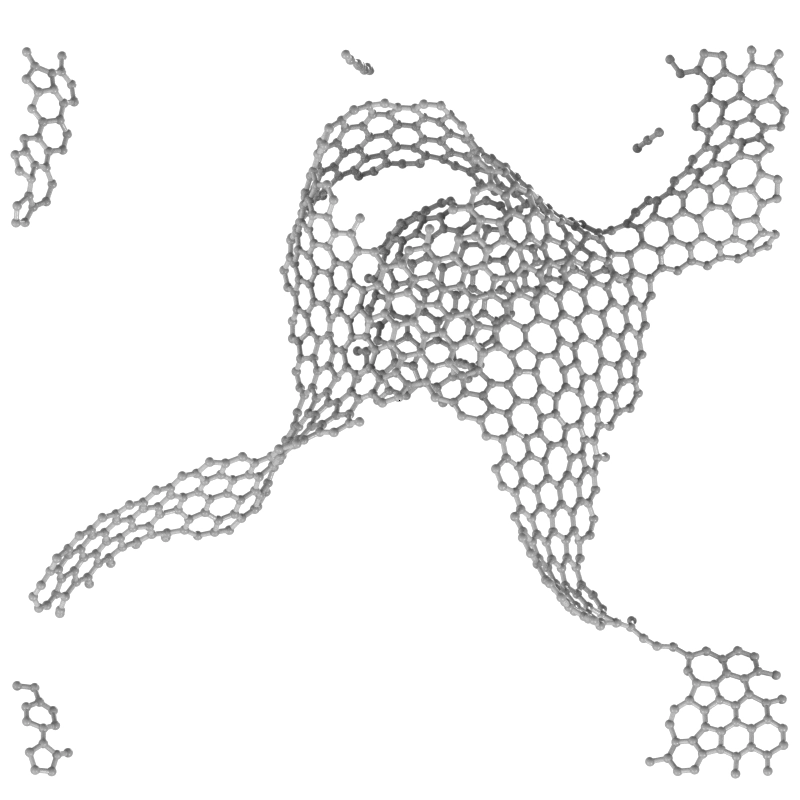
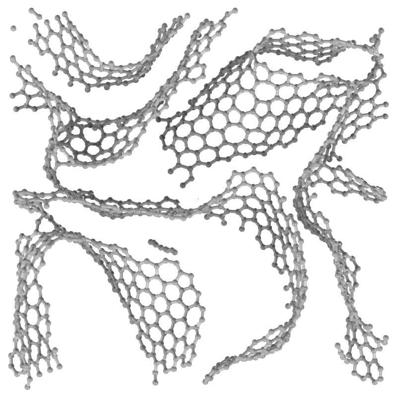
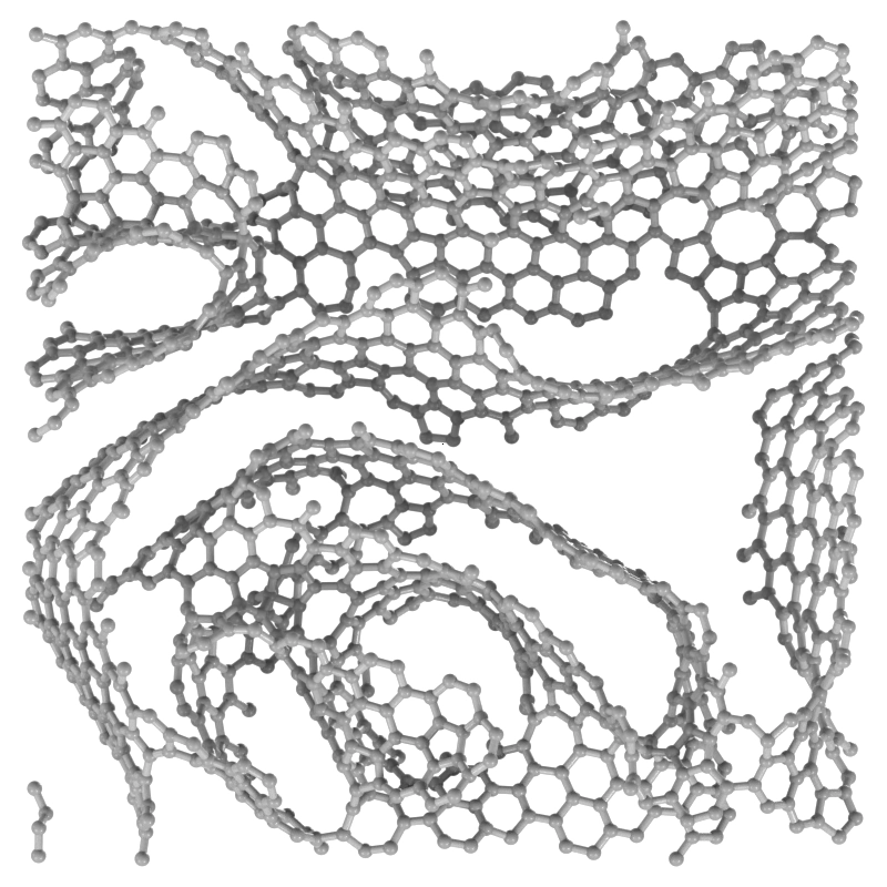
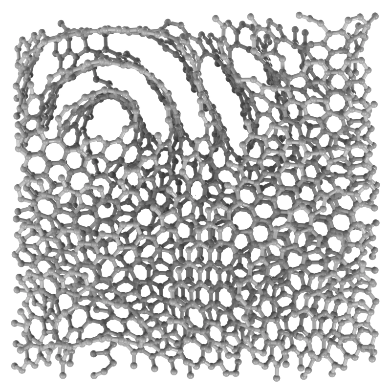
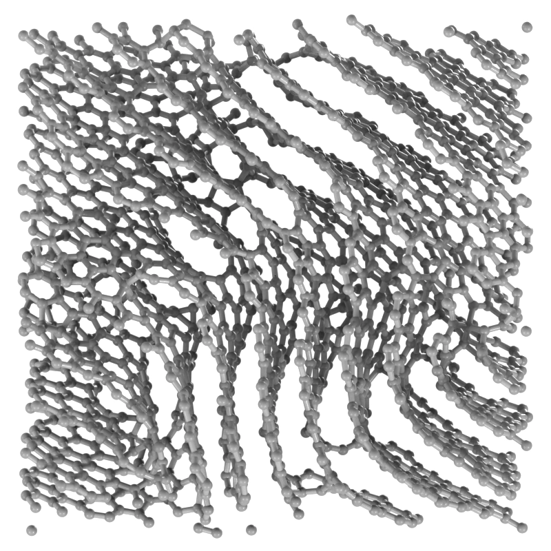
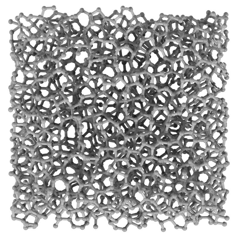
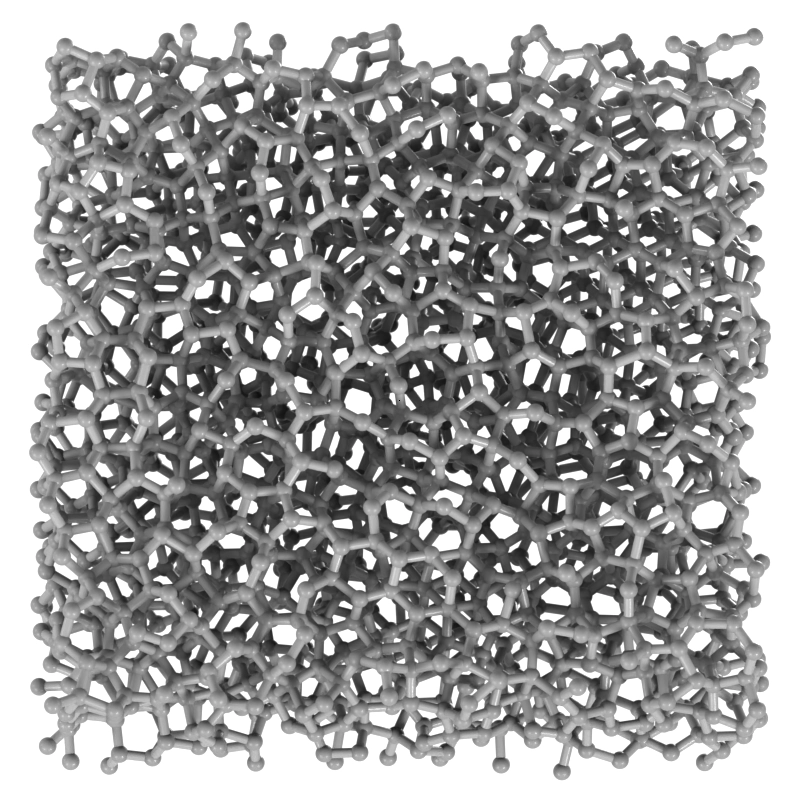
The annealed network at each density, 0.5 to 3.5 g cm⁻³, after 200 ps at 3500 K: a 10 Å slab through the final frame of replica one. All seven panels share one scale, so each cell is drawn at its true relative size: the 61.5 Å cell at 0.5 g cm⁻³ is nearly twice the width of the 32.2 Å cell at 3.5. Frames are taken at the end of each run’s cooling ramp, with no hold at 300 K.
Own work, not published elsewhere. Made with scripts/figures/render_box_grid.py.
Density sets the regime, and it does so with a switch rather than a slope. At 3500 K every density from 0.5 to 2.5 g cm⁻³ anneals to a network in which 95.8–98.6% of atoms have three neighbours: curved sheets of hexagons, wrapped round voids. At 3.0 g cm⁻³ the same anneal leaves 65.1% of atoms with four neighbours, and at 3.5 g cm⁻³, 94.8%: a dense sp³ network. The ring statistics say the same thing in a second language. Up to 2.5 g cm⁻³ six-membered rings are 66–78% of all rings, in a count of about 2,800 rings per cell; at 3.0 and 3.5 g cm⁻³ hexagons are 34.5% and 44.0% of a ring count three to four times larger, and at 3.0 g cm⁻³ five-, seven- and eight-membered rings take up most of the difference. The switch falls somewhere between 2.5 and 3.0 g cm⁻³.
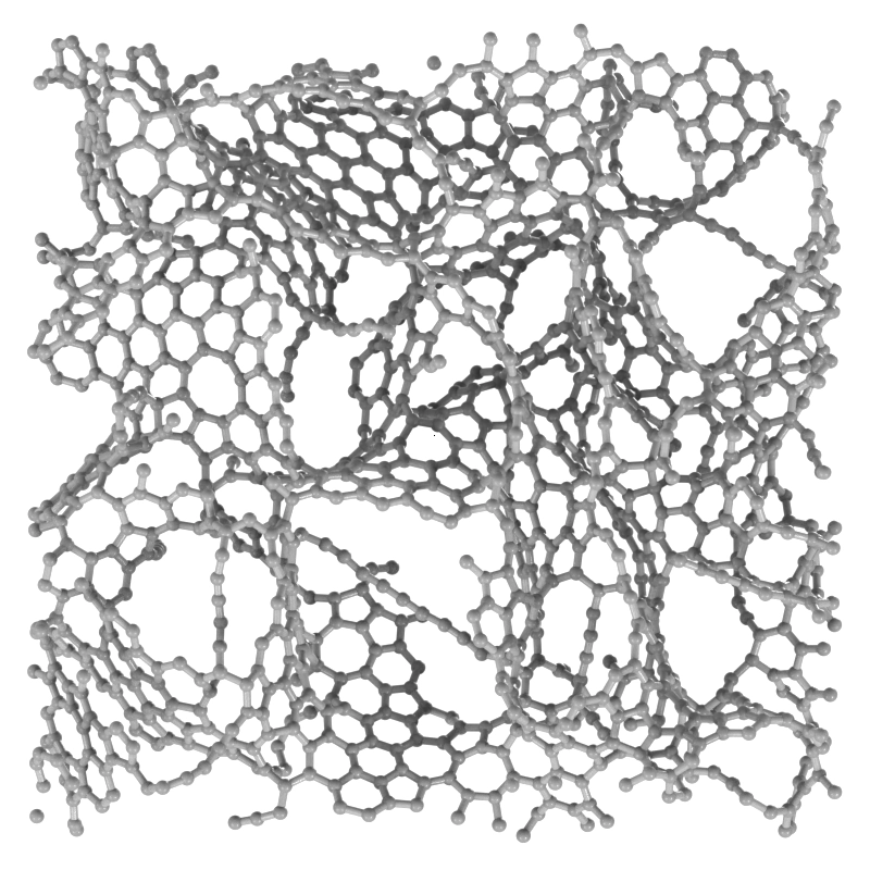
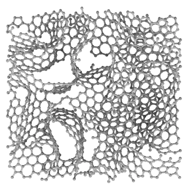
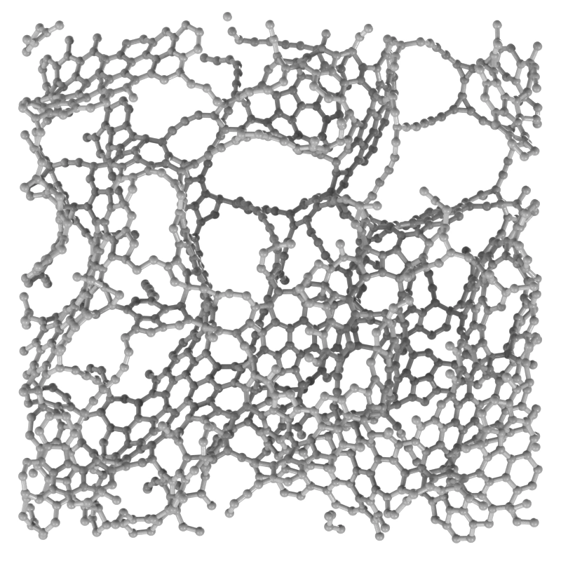
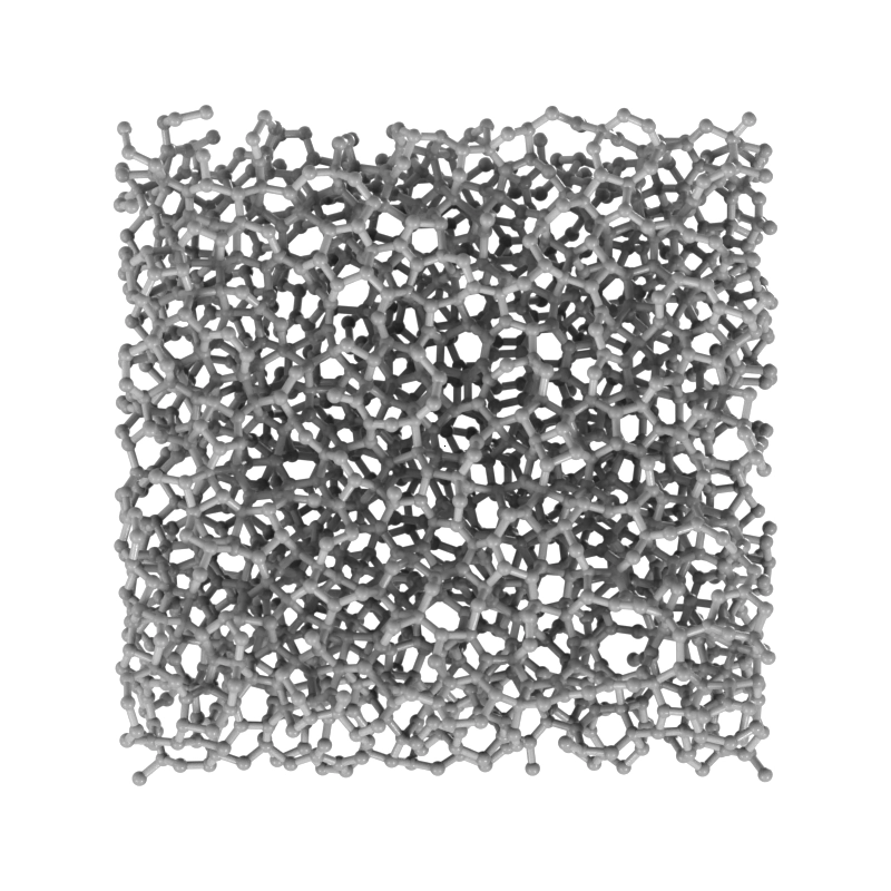
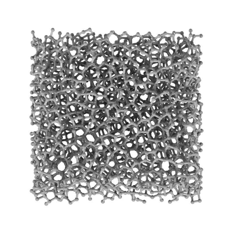
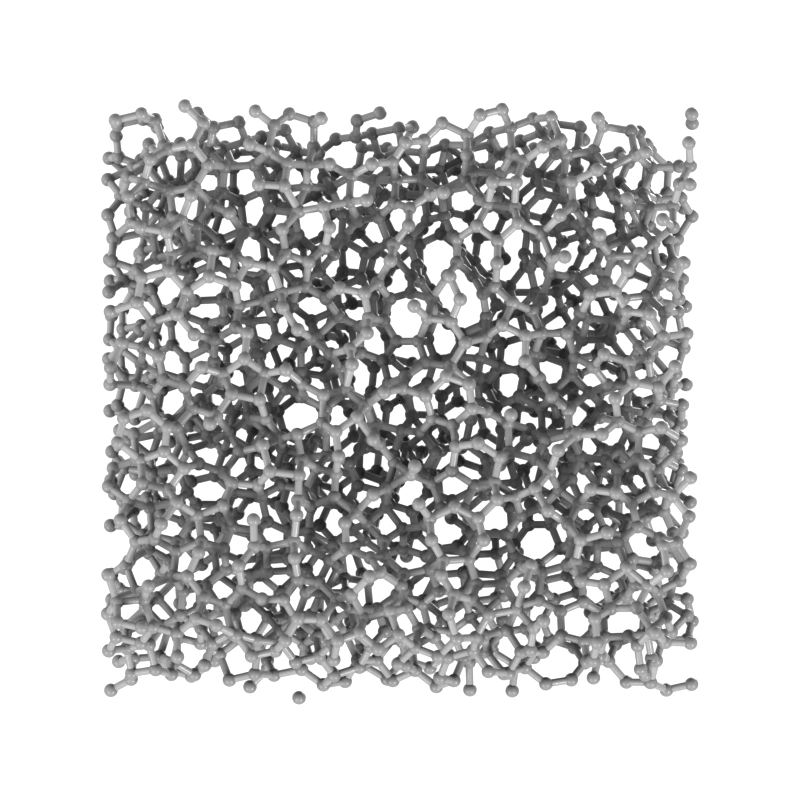
The annealed network at 2000, 3000 and 4500 K, at 1.5 g cm⁻³ (top row) and 3.0 g cm⁻³ (bottom row): 10 Å slabs through the final frame of replica one after a 200 ps anneal, every panel at one scale; the table gives all six temperatures. Frames are taken at the end of each run’s cooling ramp, with no hold at 300 K.
Own work, not published elsewhere. Made with scripts/figures/render_box_grid.py.
Temperature moves the numbers without changing the answer. At 1.5 g cm⁻³ the three-coordinated share is 89.7% at 2000 K, rises to a peak of 98.1% at 3500 K and falls to 86.0% at 4500 K, where 11.8% of atoms have been shaken loose to two neighbours; at every one of the six temperatures the material is graphitic. At 3.0 g cm⁻³ the four-coordinated share stays between 59.1% and 67.5% across 2000–4500 K; at every temperature it is a dense sp³ network. The coordination numbers behind this, averaged over the three replicas, are in the table below, and the thing to notice is that no condition in the temperature sets crosses the line that separates 2.5 from 3.0 g cm⁻³ in the density set. A 12-point swing in coordination is not nothing. But it is a change of degree inside a regime that density chose.
| Condition | Two neighbours (%) | Three neighbours (%) | Four neighbours (%) |
|---|---|---|---|
| 0.5 g cm⁻³, 3500 K | 3.7 | 95.8 | — |
| 1.0 g cm⁻³, 3500 K | — | 97.2 | — |
| 1.5 g cm⁻³, 3500 K | — | 98.1 | — |
| 2.0 g cm⁻³, 3500 K | — | 98.6 | — |
| 2.5 g cm⁻³, 3500 K | — | 97.8 | — |
| 3.0 g cm⁻³, 3500 K | — | 34.9 | 65.1 |
| 3.5 g cm⁻³, 3500 K | — | 5.1 | 94.8 |
| 1.5 g cm⁻³, 2000 K | — | 89.7 | — |
| 1.5 g cm⁻³, 2500 K | — | 94.2 | — |
| 1.5 g cm⁻³, 3000 K | — | 97.1 | — |
| 1.5 g cm⁻³, 4000 K | — | 98.0 | — |
| 1.5 g cm⁻³, 4500 K | 11.8 | 86.0 | — |
| 3.0 g cm⁻³, 2000 K | — | — | 67.5 |
| 3.0 g cm⁻³, 2500 K | — | — | 66.2 |
| 3.0 g cm⁻³, 3000 K | — | — | 59.1 |
| 3.0 g cm⁻³, 4000 K | — | — | 64.1 |
| 3.0 g cm⁻³, 4500 K | — | — | 63.9 |
The 1.0 g cm⁻³ run from liquid to annealed network, 45 seconds re-encoded from a render dated April 2021 in my archive: the 6000 K melt, the quench-and-reheat ramp, the 200 ps anneal at 3500 K and the final cooling ramp.
Own work, not published elsewhere. Made with scripts/figures/cut_graphitisation_clip.sh from the 2021 render.
Pick the density and the material will pick its bonding: that is the rule I take from this. The anneal temperature is a knob for how well-formed the sheets are and not for whether there are sheets. The caveats belong next to the rule. These are single hot frames, not averages over the anneal, and 200 ps is a long time for a potential and a short one for a kiln; the three replicas are not independent; and the coordination cutoff and ring-counting method behind the table are those of my 2021 analysis notebook, which as of September 2026 I have not re-run.
Spherical clusters
The graphitisation runs are periodic cells (boxes that repeat endlessly in every direction), carbon with no surface. The other question from the same year was about the opposite object, a free carbon nanoparticle, and which structure it settles into as a function of its size and its temperature. In early 2021 I ran 48 MD simulations of free carbon spheres to find out, eight sizes from 40 to 1,000 atoms at six temperatures from 500 to 5000 K, and this is their first appearance in public. The analysis below was redone for this page in 2026 from the archived trajectories, with a written classification rule, and it disagrees with my slides of the time in two places: the word “diamond-like”, and whether the 500 K cluster is layered at all.
Every run started from a random sphere: atoms dropped one at a time at random inside a sphere at 2.49 g cm⁻³, no two closer than 2.0 Å, with the limit relaxed slightly where placement stalled. Each size had one starting sphere, shared by all six temperatures. The sphere was relaxed briefly with the FIRE minimiser, given velocities at the target temperature and held there for 50 ps, 25,000 steps of 2 fs, under a Nosé–Hoover thermostat in LAMMPS, driven by GAP-20, as the graphitisation series was.
I analysed the last frame of every run. Two atoms are bonded if they sit closer than 1.82 Å, the cutoff the renderings on this site use, counted across the periodic boundary of the simulation cell. From that bond graph come the fraction of atoms with each number of neighbours, the connected fragments, the shortest-path rings of 3 to 10 atoms (rings with no shortcut across them), and the shells, counted as peaks in the radial density (atom density against distance from the centre) about the cluster’s centre, plus any tangentially bonded fragment nested inside. One more measure separates layered from disordered clusters: the mean absolute cosine of the angle between each bond and the radius through its midpoint, 0 for bonds lying in shells and 0.5 for bonds with no preferred direction. Run at the 1.85 Å cutoff of a Fortran ring program in the archive, the ring census reproduces, ring size for ring size, the counts that program wrote for C₁₀₀₀ at 500, 1000 and 3000 K in 2021.
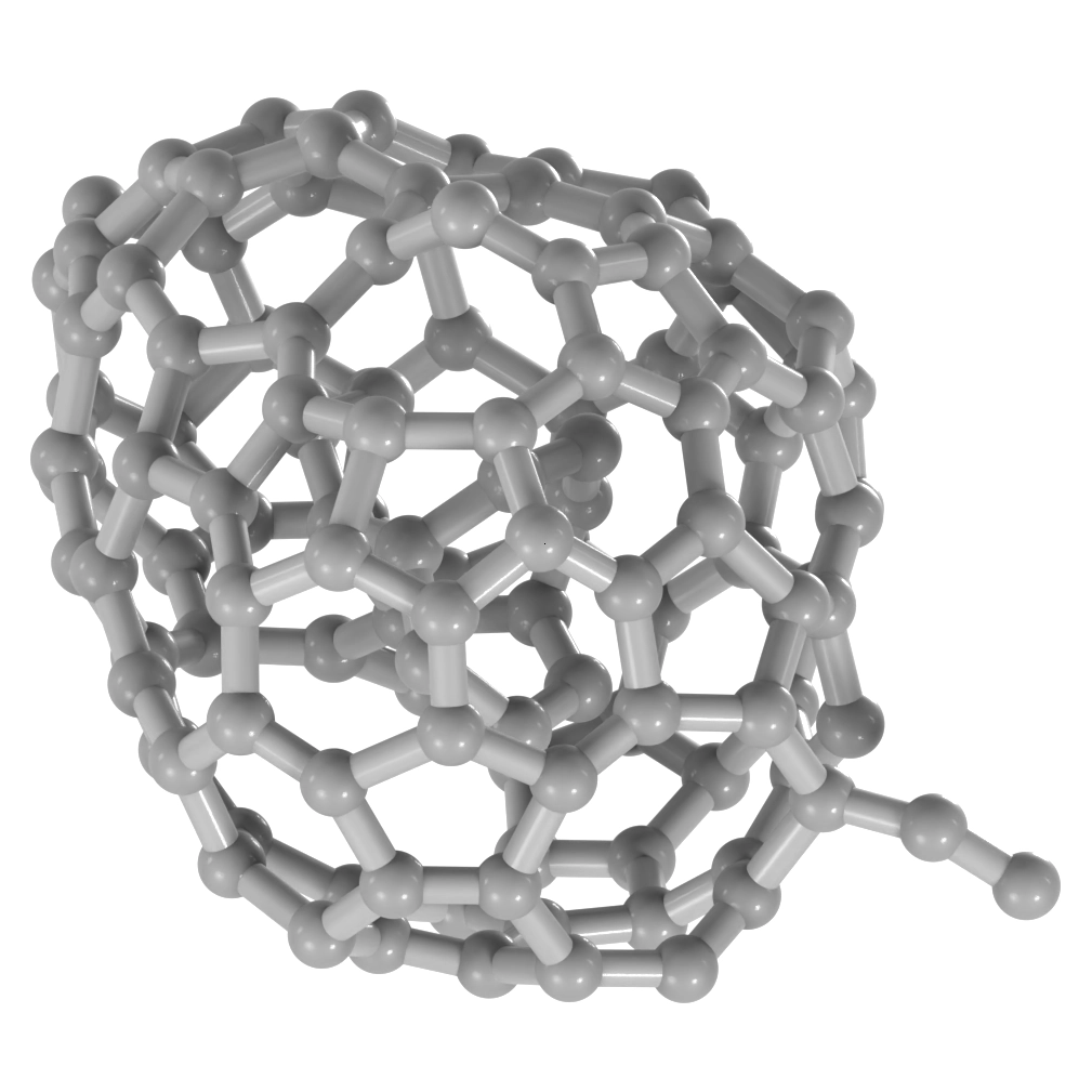
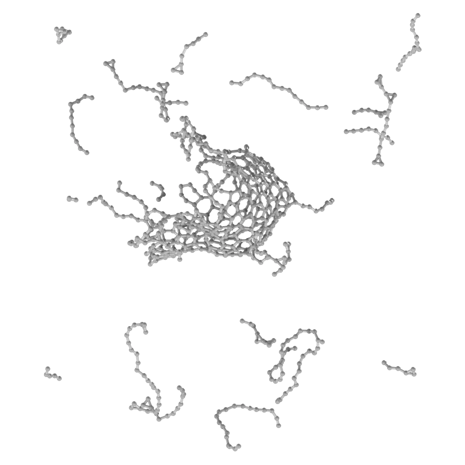
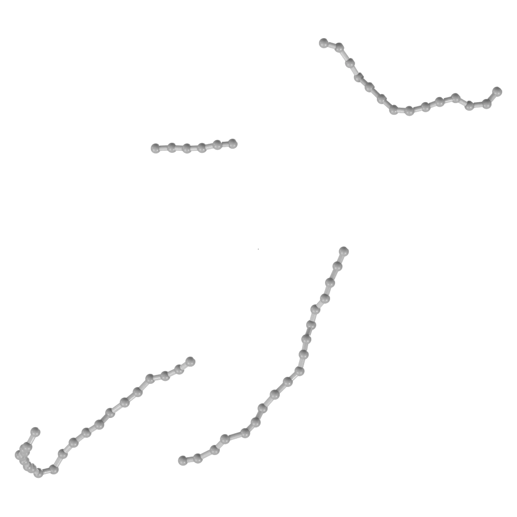
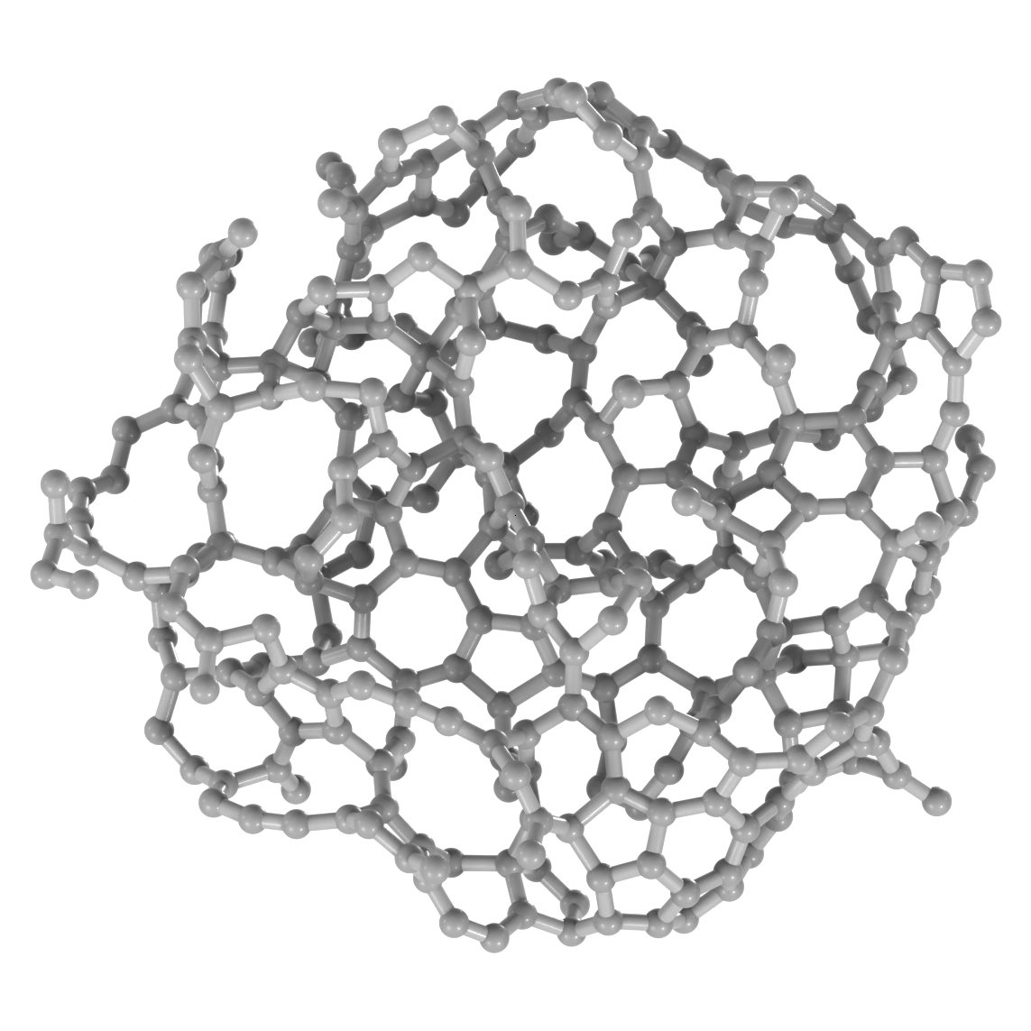
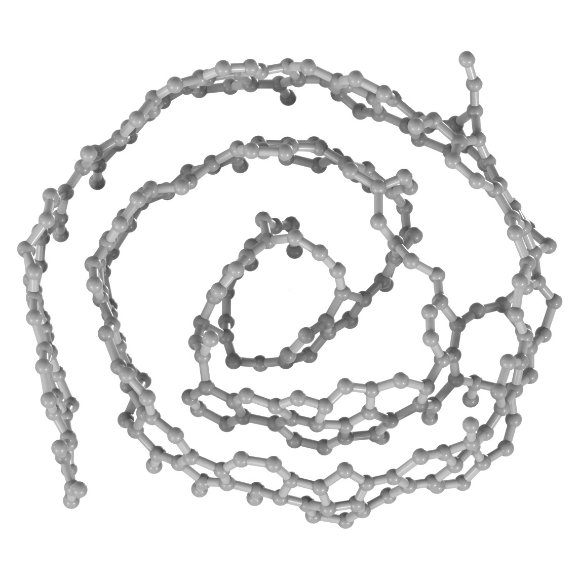
One run from each outcome class of the 48, named as the map below names them. Top, whole clusters after up to 50 ps: C₁₂₀ at 2000 K, a single closed cage; C₆₈₆ at 4000 K, the one molten run, which still held 63.8% of its atoms in one piece when it stopped at 32.9 ps; C₆₀ at 3000 K, dissociated into chains. Bottom, slices 6 Å thick through the centre of C₁₀₀₀: at 500 K the network fills the sphere with no graphitic layers, disordered; at 3000 K it has separated into three density shells, at mean radii of 4.0, 8.1 and 11.7 Å, which the slice cuts as arcs: the innermost closes, and the outer two join at one side and open at the other, so the cluster may be a scroll (one rolled-up sheet) rather than an onion. Each panel is framed to its own atoms, so sizes are not comparable between panels. Both C₁₀₀₀ runs stopped early, at 37.9 and 33.1 ps.
Own work, not published elsewhere. Made with scripts/figures/render_box_grid.py.
The outcome depends on both variables, and the pattern is simple. At 500 K every cluster holds together and none is ordered: the largest, C₁₀₀₀, is 81.3% three-coordinated, with the least layered bonding of any intact run and no graphitic layers, a disordered ball. At 1000 K the first order appears, and only in the middle sizes: C₁₂₀ closes into a cage and C₁₆₀ into an onion. At 2000 and 3000 K the clusters that survive close up into sp² shells, 84–94% of atoms three-coordinated. The small ones become single closed cages, C₆₀ to C₁₂₀ at 2000 K and C₁₂₀ and C₁₆₀ at 3000 K, and the large ones become graphitic onions of two or three nested shells, C₁₆₀ to C₁₀₀₀ at 2000 K and C₃₇₃ to C₁₀₀₀ at 3000 K. C₁₀₀₀ at 3000 K has three shells, at mean radii of 4.0, 8.1 and 11.7 Å, and 247 of its 467 rings of 3 to 10 atoms are hexagons. Heat further and the clusters come apart into carbon chains, the smallest first: C₄₀ already by 2000 K, C₆₀ and C₈₀ by 3000 K, every size but one by 4000 K and all of them at 5000 K. The one exception, C₆₈₆ at 4000 K, still held 63.8% of its atoms in one piece when its run stopped at 32.9 ps, molten rather than dissociated. Of the 48 runs, 19 dissociated, 1 was molten, 8 formed onions, 6 formed cages and 14 stayed disordered.
One symbol per run: the structure of the last frame after up to 50 ps, classified by a written rule from its coordination, fragments, shells and bond directions. No run meets the rule for diamond-like carbon, at least 40% four-coordinated atoms. Several cages and onions sit close to a class boundary; the classification notes list them.
Own work, not published elsewhere. Made with scripts/figures/cluster_outcomes.py.
Four-coordinated, diamond-like carbon never amounts to much, and this is where the analysis and my slides part company. The largest sp³ fraction in any run is 11.2%, in C₁₀₀₀ at 1000 K; at 500 K C₁₀₀₀ has 7.9%, and the smaller clusters less. Deep inside the cluster, more than 3.4 Å below the surface, C₁₀₀₀ reaches 13.9% at 500 K and 21.8% at 1000 K, and above 2000 K sp³ carbon all but disappears. In 2021 I called the 500 K C₁₀₀₀ cluster a “diamond-like sphere” with “high sp³ content”, impermeable to lithium, and contrasted it with the 3000 K onion, which was “lithium permeable”. The census supports the contrast in layering and not the word “diamond-like”, and it turns out the archive’s own ring program had printed the same 7.9% for that frame in 2021. I had the number and read the picture instead.
All 48 final frames, size across and temperature down
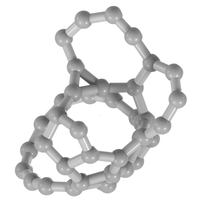
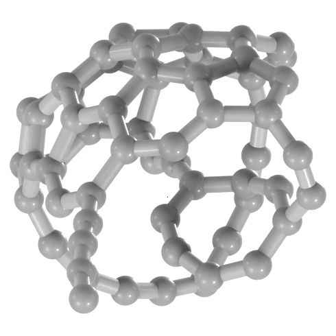
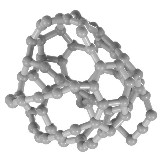
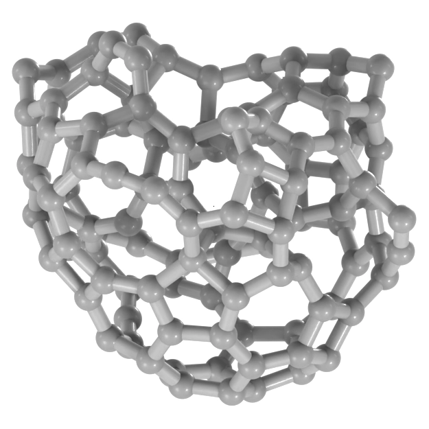
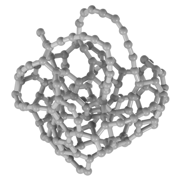
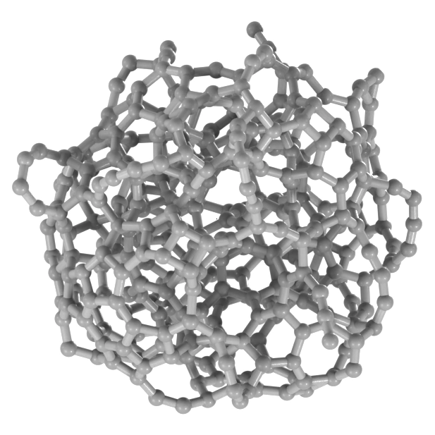
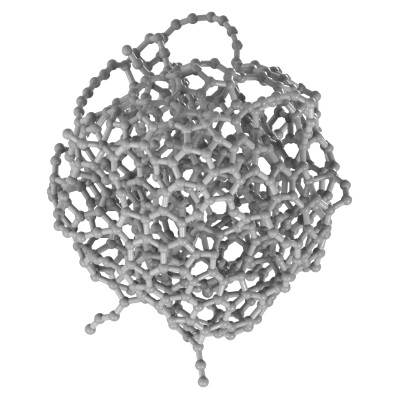
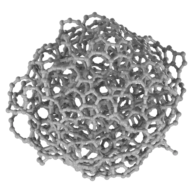
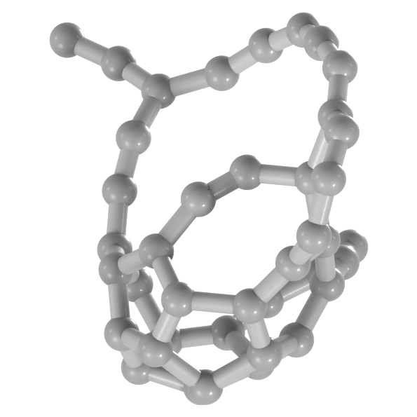
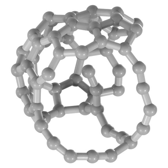
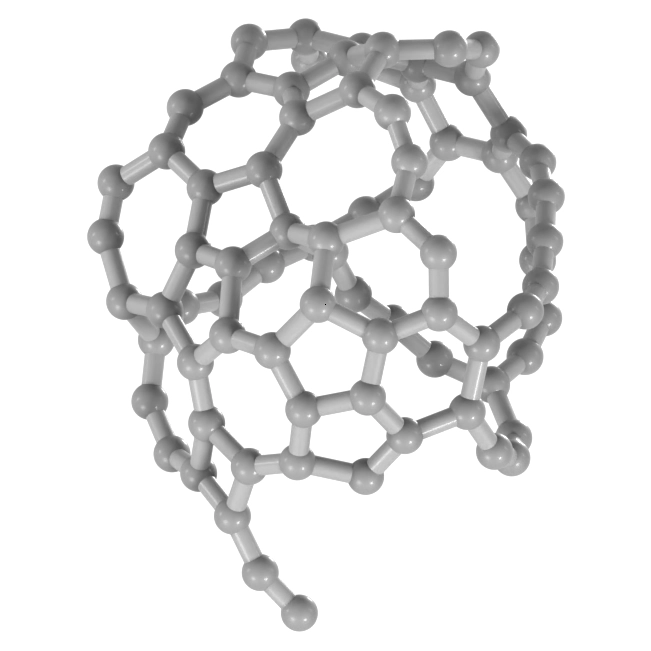
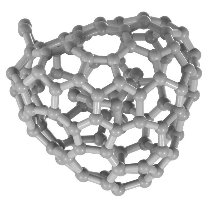
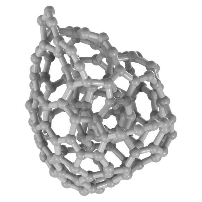
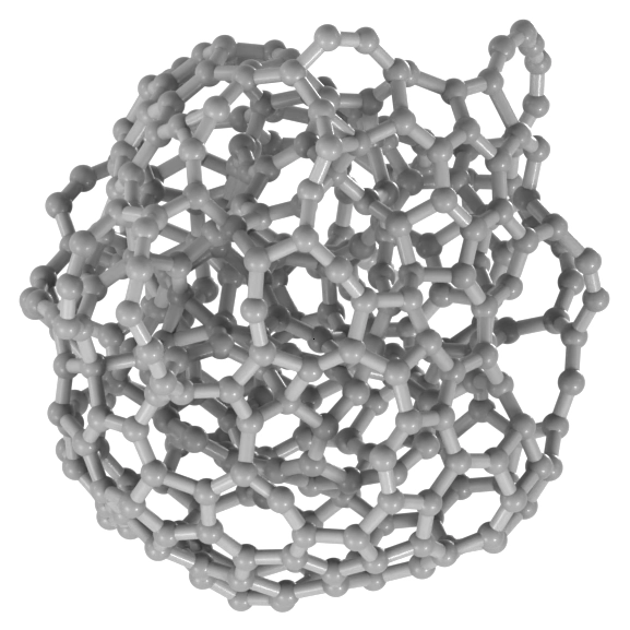
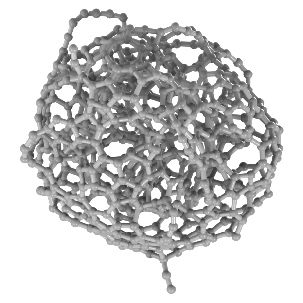
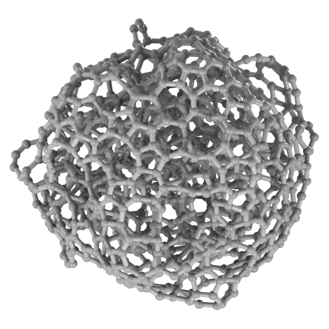
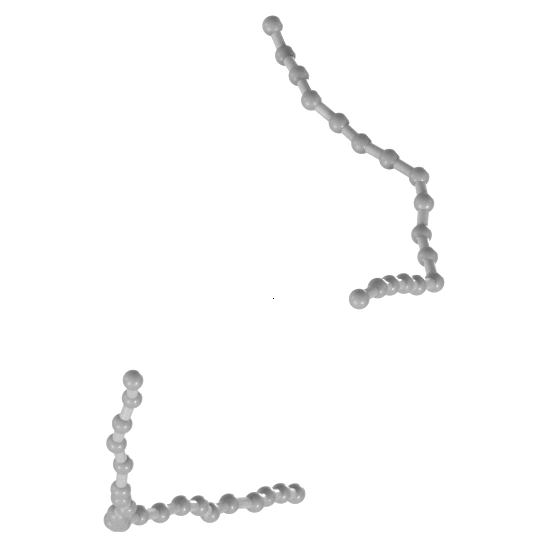
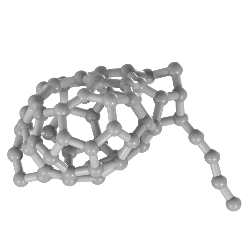
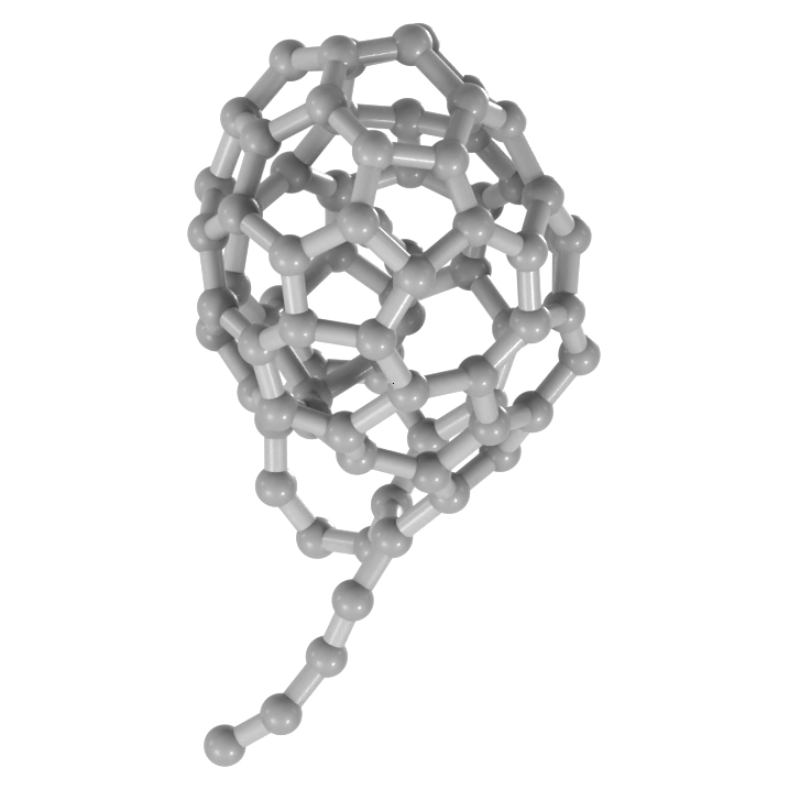
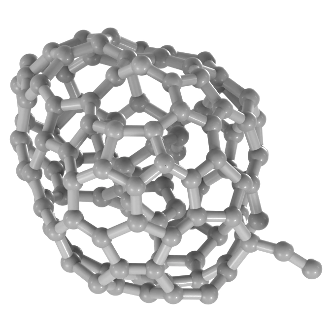
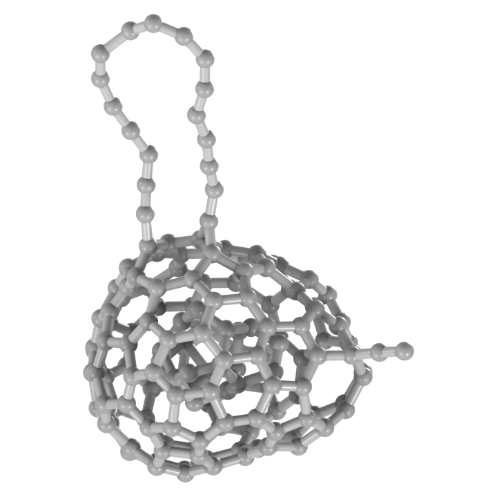
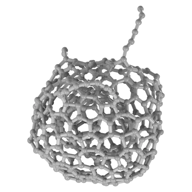
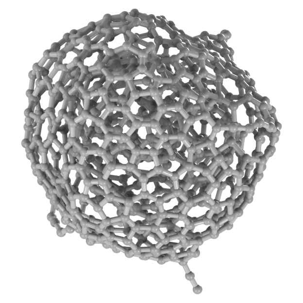
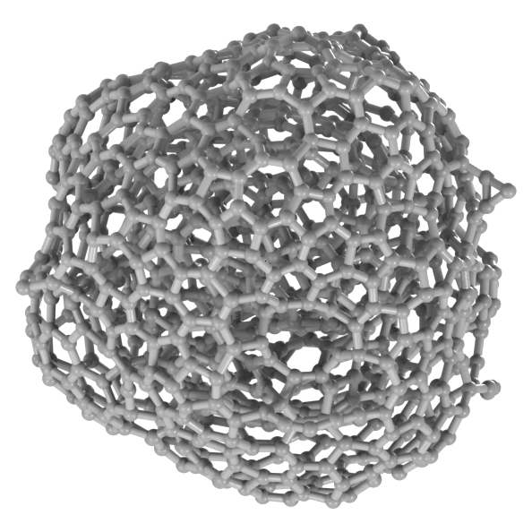
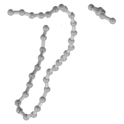
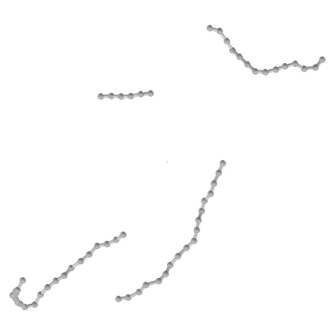
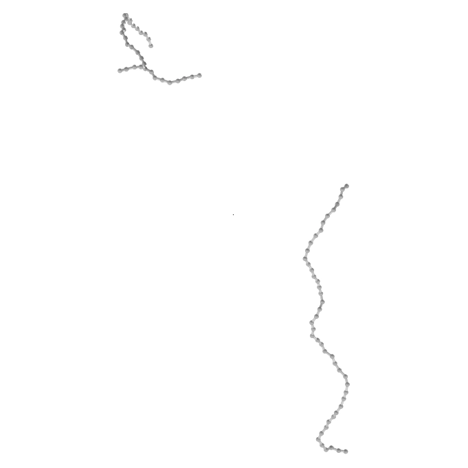
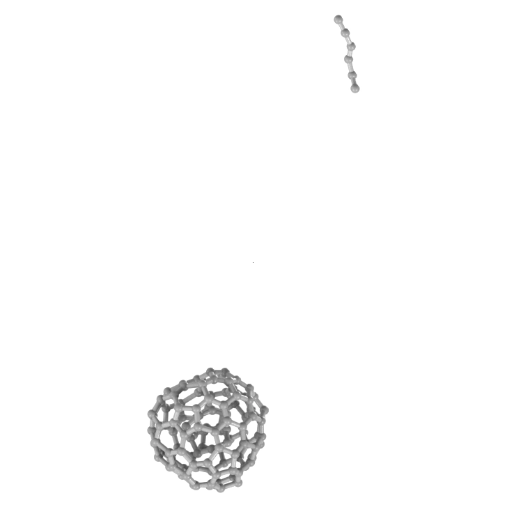
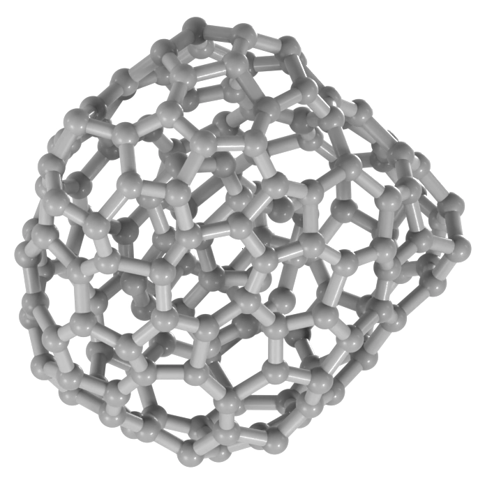
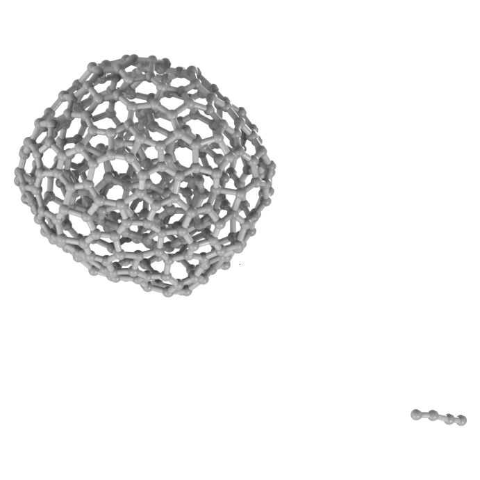
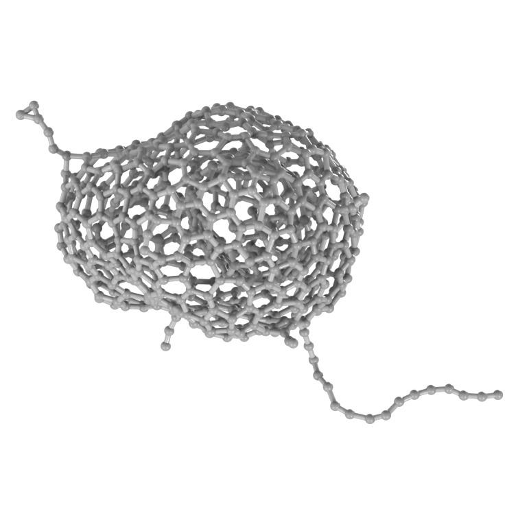
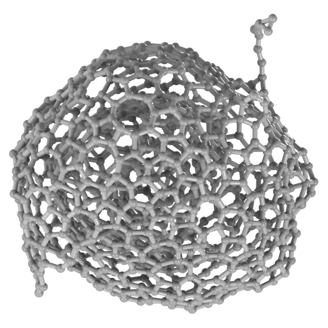
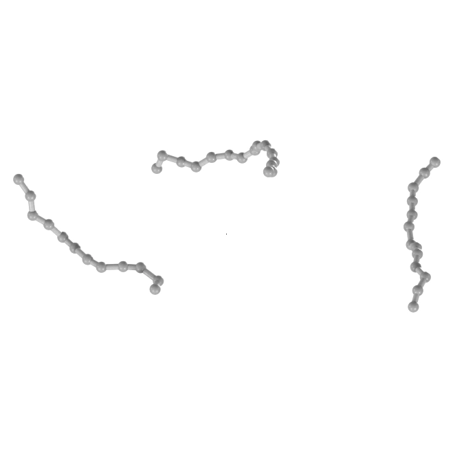
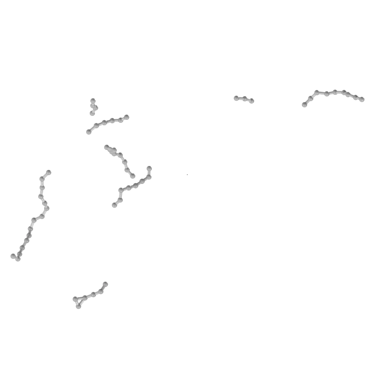
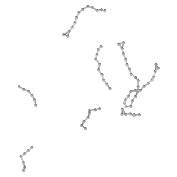
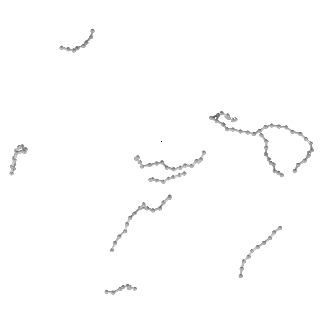
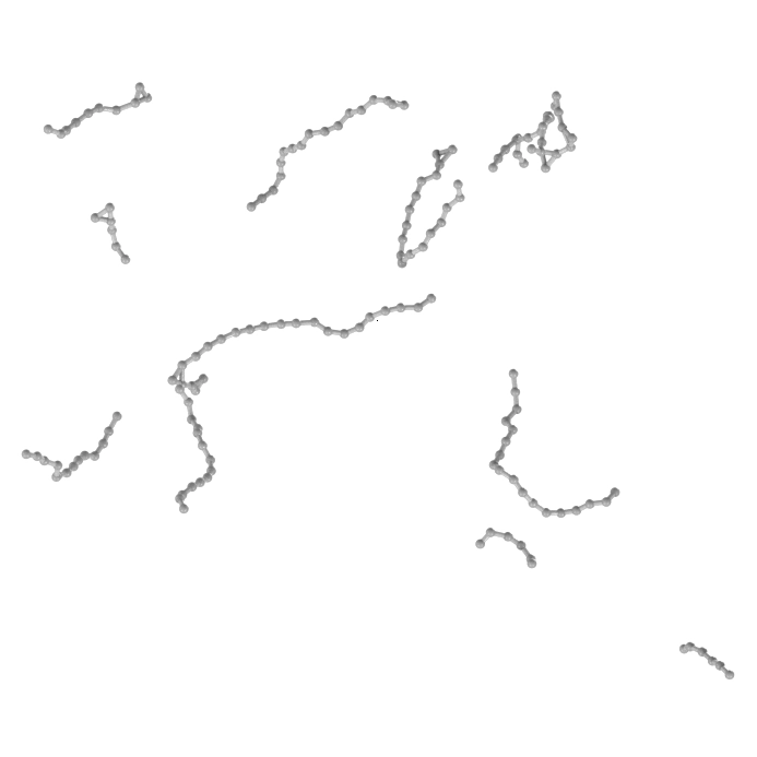
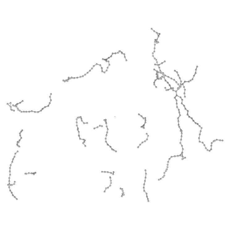
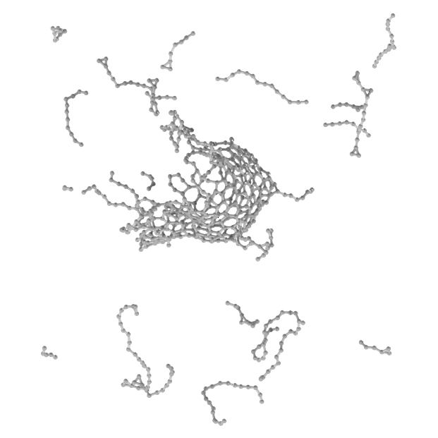
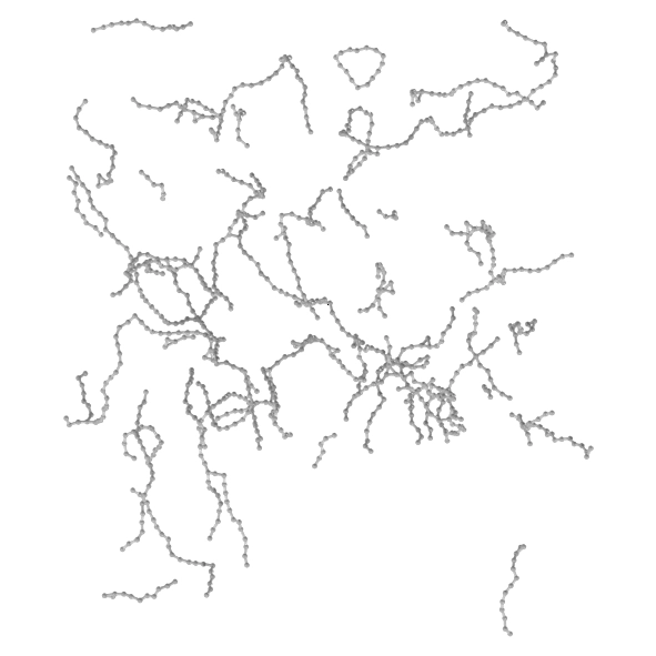
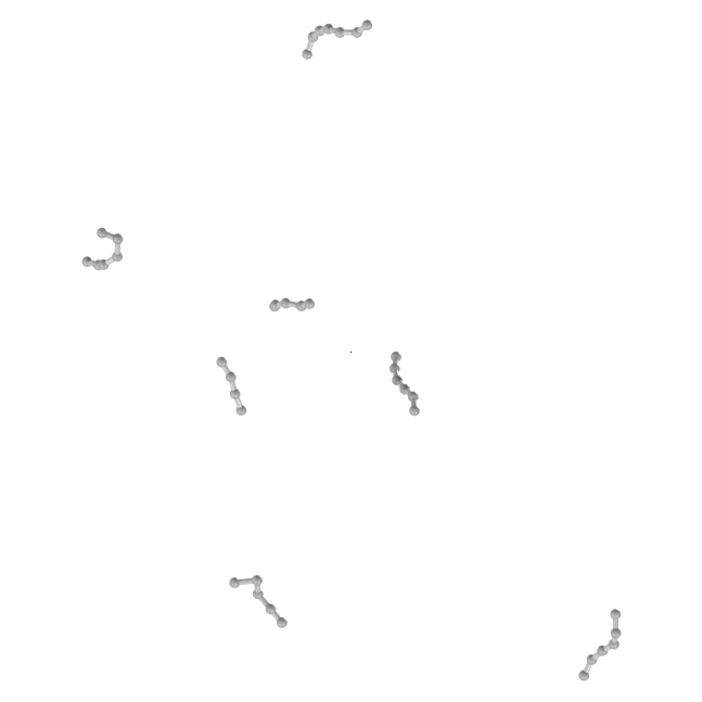
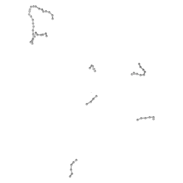
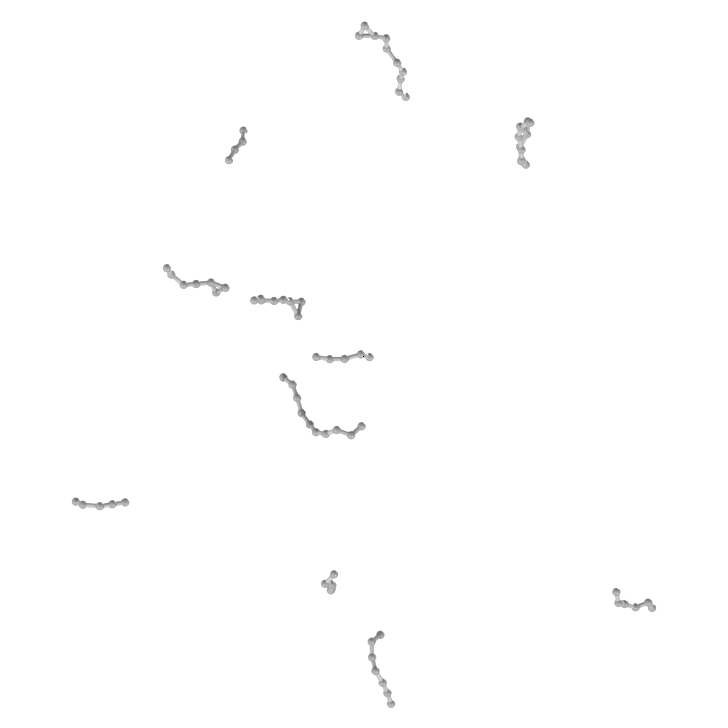
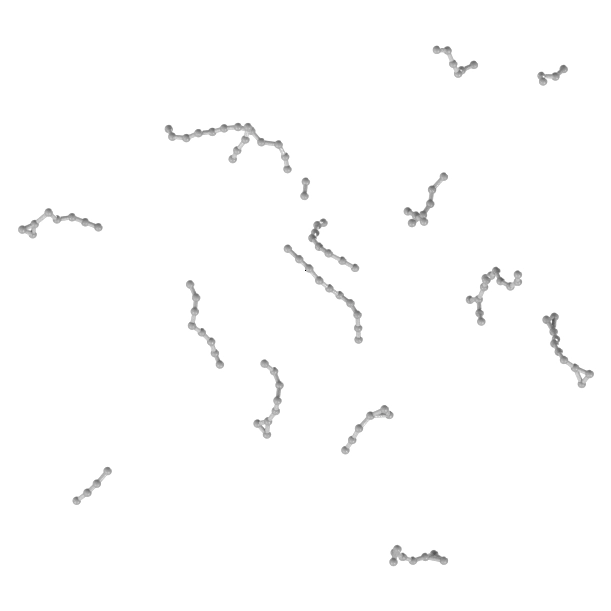
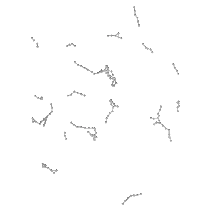
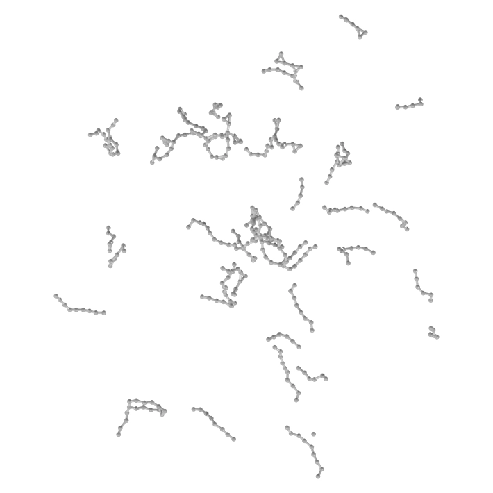
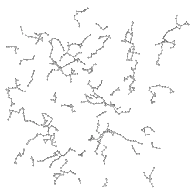
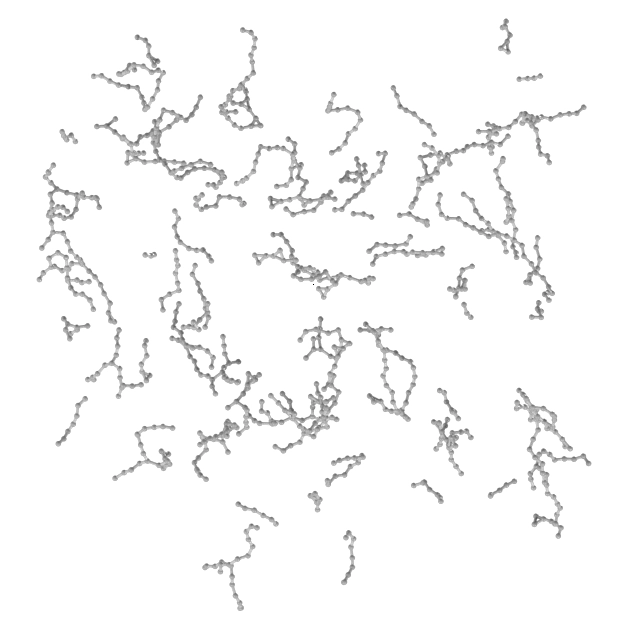
The last frame of every run, for the record: eight sizes across, six temperatures down, each panel framed to its own atoms, so sizes are not comparable between panels. Open the list to see them; a panel enlarges on a click. Ten runs stopped before 50 ps (all six C₁₀₀₀ runs; C₆₈₆ at 1000, 3000 and 4000 K; C₈₀ at 500 K), and the C₈₀ and C₆₈₆ panels at 500 K are byte-identical copies of two earlier test runs that were relaxed with a different minimiser from the rest.
Own work, not published elsewhere. Made with scripts/figures/render_box_grid.py.
The map has limits. Each cell is one frame of one trajectory, not an average and not a converged phase: there are no replicas, one starting structure per size and 50 ps at most. Ten runs stopped early, between 29.9 and 49.8 ps, including all six C₁₀₀₀ runs, and two of the 500 K runs, C₈₀ and C₆₈₆, were relaxed with a different minimiser from the rest. Several of the cages and onions sit near a class boundary, C₁₆₀ at 2000 K most of all, with a 20-atom cage nested inside a 140-atom one, and a count of density shells cannot tell an onion from a scroll. What survives all of that is the shape of the map. Cold clusters are disordered, warm ones are cages and onions, hot ones are chains, and up to C₆₈₆ the temperature at which a cluster stops being a cluster rises with its size.
CHO-GAP
Carbon is rarely found alone, and my thesis names hydrogen and oxygen as the next step for that reason: the char in a furnace, the hard carbon in a battery anode and the soot in a flame all carry both. The GAP-20 paper lists hydrogenation and oxidation among the things it cannot do. So the last carbon potential I worked on was CHO-GAP (carbon, hydrogen and oxygen): the same method, three elements. This section is shorter than the work was, because the project ended without a paper and the numbers I would like to give you are in a draft and a set of status notes that as of September 2026 I have not put beside this page, so they stay off it. What I can show is what the data files on this site show.
Eight methane and sixteen oxygen molecules in a 10 Å periodic box at 3000 K under CHO-GAP, at 0, 10, 20 and 50 ps, drawn as ball-and-stick monochrome with carbon filled, oxygen open and hydrogen small. At 50 ps the box holds 7 CO₂, 1 CO, 12 H₂O, 3 OH, 3 H and 1 H₂O₂: methane has burned, with the radicals (reactive fragments such as OH and H) a flame is supposed to have.
Own work, not published elsewhere. Made with scripts/figures/combustion_frames.py and scripts/figures/render_cluster.py.
The model was built the way the thesis says to build one, and one demonstration of it is worth the space. A 10 Å box held 8 CH₄ and 16 O₂ at 3000 K for 50 ps. At the end it held 7 CO₂, 1 CO, 12 H₂O, 3 OH, 3 H and 1 H₂O₂. That is combustion, complete with the radicals, from a potential that was fitted to energies and forces and was never told what a reaction is. It is a sanity check rather than a validation, since no one measured the reaction rates in the box against anything, but a potential that gets combustion qualitatively wrong would show it here, and this one does not.
The project ran with Carla de Tomas and Cedric Weber at Happy Electron and KCL, Jean-Marc Leyssale in Bordeaux, who analysed frames from lignin pyrolysis (the heating of lignin, a wood polymer, without oxygen) with it, and Gábor Csányi. It ended because the technology moved on. In 2022 Csányi’s group published MACE, a machine-learned potential built as a neural network rather than a Gaussian-process fit; it was clearly a step change in performance, and we chose to move to it rather than finish a model of the generation before. A potential that works is a model; finished work is a model, its limits understood, and a paper that says both, and CHO-GAP was set aside before its paper was finished. The lesson of the whole page, if it has one, is that the second of those is the part you cannot let the computer decide.
Publications in this article
- 2022
B. Karasulu, J.-M. Leyssale, P. Rowe, C. Weber, C. de Tomas. Accelerating the prediction of large carbon clusters via structure search: evaluation of machine-learning and classical potentials. Carbon 191, 255–266.
- 2021
F. L. Thiemann, P. Rowe, A. Zen, E. A. Müller, A. Michaelides. Defect-dependent corrugation in graphene. Nano Lett. 21, 8143–8150.
- 2020
- 2018
P. Rowe, G. Csányi, D. Alfè, A. Michaelides. Development of a machine learning potential for graphene. Phys. Rev. B 97, 054303.